
California Greenhouse Gas Emissions
for 2000 to 2020
Trends of Emissions and Other Indicators
Date of Release: October 26, 2022
California Air Resources Board
1001 I Street
Sacramento, California 95814

Executive Summary
The annual statewide greenhouse gas (GHG) emission inventory is one tool to track progress of
California’s climate programs toward achieving the statewide GHG goals. This document
summarizes the trends in emissions and indicators in the California GHG Emission Inventory (“the
GHG Inventory”). The emissions included in the inventory and presented here represent actual
emissions released into the atmosphere from the AB 32 sectors. The 2022 edition of the inventory
includes GHG emissions released during 2000-2020 calendar years and includes several technical
updates. For some sectors, these changes are substantial and impact the entire time series. Details
on these updates are described in more detail in the technical documentation
a
available on GHG
Inventory program website at: https://ww2.arb.ca.gov/ghg-inventory-data.
In 2020, emissions from GHG emitting activities statewide
b
were 369.2 million metric tons of
carbon dioxide (CO
2
) equivalent (MMTCO
2
e), 35.3 MMTCO
2
e lower than 2019 levels and 61.8
MMTCO
2
e below the 2020 GHG Limit of 431 MMTCO
2
e. The 2019 to 2020 decrease in emissions is
likely due in large part to the impacts of the COVID-19 pandemic. Economic recovery from the
pandemic may result in emissions increases over the next few years. As such, the total 2020
reported emissions are likely an anomaly, and any near-term increases in annual emissions should
be considered in the context of the pandemic. The most notable highlights in the 2022 edition
inventory include:
• The transportation sector showed the largest decline in emissions of 27 MMTCO
2
e (16
percent) compared to 2019. This decrease was most likely from light duty vehicles after
shelter-in-place orders were enacted in response to the COVID-19 pandemic.
• Industrial sector emissions dropped 7 MMTCO
2
e (9 percent) compared to 2019. The
decrease is driven by lower emissions from both the refining sector and the oil and gas
production sector.
• Electricity sector emissions remained at a similar level as in 2019 despite a 44 percent
decrease in in-state hydropower generation (due to below average precipitation levels),
which was more than compensated for by a 10 percent growth in in-state solar generation
and cleaner imported electricity incentivized by California’s clean energy policies.
• Between 2019 and 2020, California’s Gross Domestic Product (GDP) contracted 2.8 percent
while the GHG intensity of California’s economy (GHG emissions per unit GDP) decreased
6.2 percent.
a
Inventory Updates Since the 2021 Edition of the Inventory - Supplement to the Technical Support Document.
Available at: https://ww2.arb.ca.gov/sites/default/files/classic/cc/inventory/ghg_inventory_00-
20_method_update_document.pdf
b
Pursuant to the California Global Warming Solutions Act (Assembly Bill 32, or “AB 32”), the GHG Inventory includes
emissions from in-state sources and imported electricity, emissions of which were released from electricity
generation facilities located outside of California.
2

Figure 1. Compares Annual Statewide GHG Emissions to the 2020 GHG Limit.
This graph shows California’s annual GHG emissions from 2000 to 2020 in relation to the 2020 GHG Limit required by
the California Global Warming Solutions Act (Assembly Bill 32) [1]. Emissions were 431.5 in 2013, and in 2014,
California’s GHG emissions dropped below the 2020 GHG Limit and have remained below the 2020 GHG Limit since
that time.
3

Introduction
The GHG Inventory is one tool to track the State’s progress toward achieving the statewide GHG
goals established by Assembly Bill 32 (AB 32) (reduce emissions to 1990 levels by 2020) and
Senate Bill 32 (SB 32) (reduce emissions to at least 40 percent below 1990 levels by 2030). The
GHG Inventory includes the following types of sources: emissions from fossil fuel combustion,
including combustion for imported electricity consumed in state, GHGs generated as by-products
of chemical reactions in industrial processes, use of GHG-containing consumer products and
human-made chemicals, and emissions from agricultural and waste sector operations. The
exchange of ecosystem carbon between the atmosphere and the plants and soils in land is
separately quantified in the Natural and Working Lands Ecosystem Carbon Inventory [2], which
also includes the amount of carbon impacted by wildfire. For the emission sources included in the
GHG Inventory, the inventory framework is consistent with international and national GHG
inventory practices [3], and is aligned with requirements in AB 32.
The 2022 edition of the GHG Inventory includes the emissions of the seven GHGs identified in
AB 32 [1] for the years 2000 to 2020. There are additional climate pollutants that are not included
in AB 32 that are tracked separately outside of the GHG Inventory. These climate pollutants
include black carbon and sulfuryl fluoride (SO
2
F
2
), which are discussed in the Short-Lived Climate
Pollutant (SLCP) Strategy [4], and ozone depleting substances (ODS), which are being phased out
under a 1987 international treaty [5]. ODSs are now being substituted with hydrofluorocarbons,
which are pollutants specified in AB 32 [1].
In this report, emission trends and indicators are presented in the categories outlined in the Initial
AB 32 Climate Change Scoping Plan [6]. There are alternative ways of organizing emission sources
into categories, and the resulting percentages will be different depending on these categorization
schemes. The Additional Information section at the end of this report provides further information
on alternative categorization schemes. All emissions in this report are expressed in 100-year
Global Warming Potential (GWP) from the Intergovernmental Panel on Climate Change (IPCC) 4th
Assessment Report (AR4)[7], consistent with current international GHG inventory practices.
Statewide Trends of Emissions and Indicators
In 2020, emissions from statewide emitting activities were 369.2 million metric tons of CO
2
equivalent (MMTCO
2
e, or million metric tons CO
2
e), 35.3 MMTCO
2
e lower than 2019 levels and
61.8 MMTCO
2
e below the 2020 GHG Limit of 431 MMTCO
2
e. Since the peak level in 2004,
California’s GHG emissions have generally followed a decreasing trend. In 2014, statewide GHG
emissions dropped below the 2020 GHG Limit and have remained below the Limit since that time.
c
Per capita GHG emissions in California have dropped from a 2001 peak of 13.8 metric tons per
person to 9.3 metric tons per person in 2020, a 33 percent decrease [8][9]. Overall trends in the
c
Previous editions of this report indicated that total emissions dropped below the 2020 GHG Limit in 2016. The
technical refinements implemented in the 2022 edition inventory resulted in updates to emissions data for previous
years. The updated inventory indicates that emissions dropped below the 2020 GHG Limit in 2014.
4

inventory also continue to demonstrate that the carbon intensity of California’s economy (the
amount of carbon pollution per million dollars of gross domestic product (GDP)) is declining.
From 2000 to 2020, the carbon intensity of California’s economy decreased by 49 percent while
the GDP increased by 56 percent. Likely in part due to the COVID-19 pandemic, GDP fell 2.8
percent in 2020 while the emissions per GDP declined by 6.1 percent compared to 2019 [8][10].
Figures 2(a)-(c) show these economic indicators alongside GHG emissions.
Figure 2a. Change in California GDP, Population, and GHG Emissions Since 2000.
Metric Associated 2020 Value
GDP 2.7 trillion (2012 $)
Population 39.5 million
GHG Emissions 369.2 MMTCO
2
e
GHG Emissions per Capita 9.3 metric tons CO
2
e per person
GHG Emissions per GDP 139 metric tons CO
2
e per million $
5


Overview of Emission Trends by Sector
The large decline in total statewide 2020 emissions is likely due in large part to the impact of the
COVID pandemic. Additional drivers of emission changes are noted for each sector below. The
transportation sector remains the largest source of GHG emissions in the State. Direct emissions
from vehicle tailpipes, off-road transportation sources, intrastate aviation, and other
transportation sources, account for 37 percent
d
of statewide emissions in 2020. This is a smaller
share than recent years, as the transportation sector saw a significant decrease of 26.6 MMTCO
2
e
in 2020. When upstream emissions from oil extraction, petroleum refining, and oil pipelines in
California are included, transportation is responsible for about 47 percent of statewide emissions
in 2020. Emissions from the electricity sector account for 16 percent of the inventory in 2020 and
had a slight decrease of 0.7 MMTCO
2
e compared to 2019. Continued growth in in-state solar
generation and increases in imported renewable electricity more than compensate for the
significant drop in in-state hydropower generation due to below average precipitation levels. The
industrial sector trend has been relatively flat in recent years but saw a decrease of 7.1 MMTCO
2
e
in 2020. Commercial & residential emissions saw a decrease of 1.7 MMTCO
2
e. Emissions from
high-GWP gases have continued to increase as they replace ODS that are being phased out under
the 1987 Montreal Protocol [5]. Emissions from other sectors have remained relatively constant
in recent years. Figure 3 shows an overview of the emission trends by Scoping Plan sector. Figure
4 breaks out 2020 emissions by sector into an additional level of sub-sector categories.
d
The transportation sector represents tailpipe emissions from on-road vehicles and direct emissions from other off-
road mobile sources. It does not include upstream well-to-tank emissions from oil extraction, petroleum refining, and
oil pipelines. These upstream emissions are included in the industrial sector category.
7
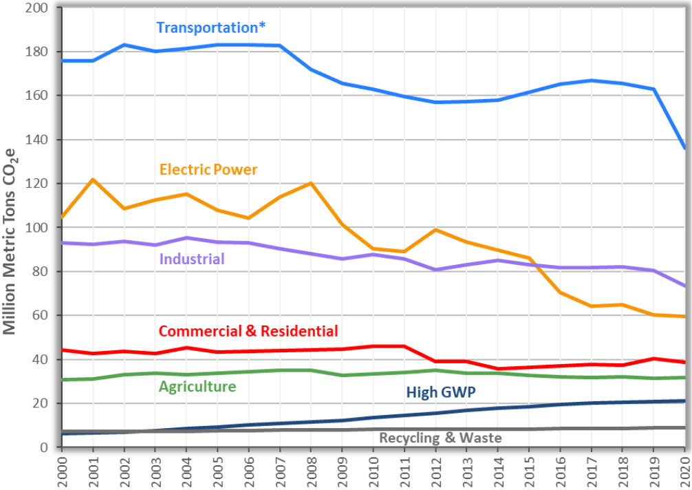
Figure 3. Trends in California GHG Emissions.
This figure shows changes in emissions by Scoping Plan sector between 2000 and 2020. Emissions are organized by
the categories in the AB 32 Scoping Plan.
*The transportation sector represents tailpipe emissions from on-road vehicles and direct emissions from other off-
road mobile sources. It does not include upstream well-to-tank emissions from oil extraction, petroleum refining, and
oil pipelines. These upstream emissions are included in the industrial sector category.
8
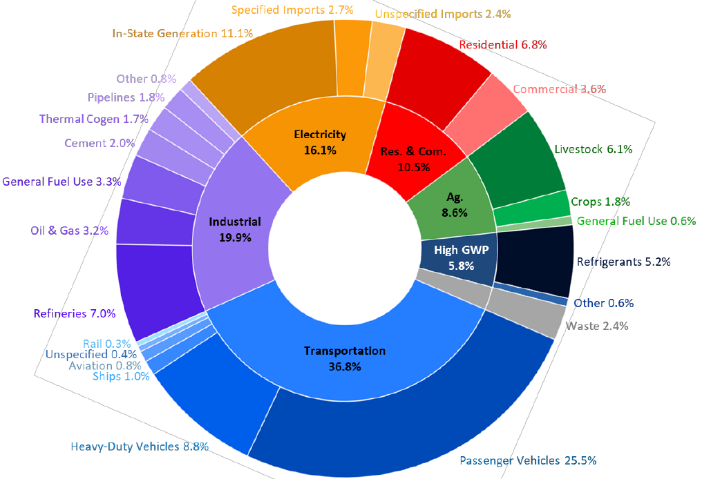
Figure 4. 2020 GHG Emissions by Scoping Plan Sector and Sub-Sector Category.
*
This figure breaks out 2020 emissions by sector into an additional level of sub-sector categories. The inner ring shows
the broad Scoping Plan sectors. The outer ring breaks out the broad sectors into sub-sectors or emission categories
under each sector.
*The transportation sector represents tailpipe emissions from on-road vehicles and direct emissions from other off-
road mobile sources. It does not include emissions from petroleum refineries, oil extraction and production, and oil
pipelines, which are included in the industrial sector.
9

Transportation
The transportation sector remains the largest source of GHG emissions in 2020, accounting for
37 percent
e
of California’s GHG inventory in 2020, a drop from 40 percent in 2019. Contributions
from the transportation sector
f
include emissions from combustion of fuels in State that are used
by on-road and off-road vehicles, aviation, rail, and water-borne vessels, as well as a few other
smaller sources. (In this report, emissions from refrigerants used in vehicles, airplane, train, and
ship and boat are shown in the high-GWP gases category.) A combination of factors influences
transportation emissions. Fuel policies (such as policies that incentivize low-carbon fuels),
improved fuel efficiency of the State’s vehicle fleet, and higher market penetration of zero-
emission vehicles can drive down consumption and emissions over time. Year-to-year changes in
economic conditions can also impact the amount of transportation fuel used across the state.
In early 2020, the COVID-19 pandemic had wide-ranging impacts on people and economies
around the world. In California, the measures put into place to slow the spread of COVID-19
resulted in substantial changes in human and vehicle activity. Most notably, significant reductions
in heavy-duty and light-duty vehicle miles traveled (VMT) across the State’s highways and local
roads resulted in a steep decline in transportation emissions. Statewide VMT was found to fall to
its lowest point in April 2020, when heavy-duty VMT was 13 percent lower and light-duty VMT
was 44 percent lower than in April 2019. In the months following, both heavy-duty and light-duty
VMT increased, with heavy-duty VMT returned and surpassed levels observed in 2019 by the end
of 2020, as the demand for goods movement increased [11].
Emissions from transportation sources peaked from 2002 to 2007, then steadily decreased until
2012, when transportation sector emissions began to rise again. Emissions from this sector have
declined for three consecutive years since 2017 with 2020 having the largest emission change
g
, a
decrease of 26.6 MMTCO
2
e in one year. Figure 5 shows an overview of GHG emissions from the
transportation sector.
e
The 37 percent figure represents tailpipe emissions from on-road vehicles and direct emissions from other non-road
transportation sources. It does not include upstream well-to-tank emissions from oil extraction, petroleum refining,
and oil pipelines, which are included in the industrial sector.
f
Emissions from the following sources are not included in the GHG inventory for the purpose of comparing to the GHG
Limit, but are tracked separately as informational items and are published with the GHG inventory: interstate and
international aviation, diesel and jet fuel use at military bases, and a portion of bunker fuel purchased in California
that is combusted by ships beyond 24 nautical miles from California’s shores. The following emissions are not
included or tracked in the GHG inventory: emissions from the combustion of fuels purchased outside of California that
are used in-state by passenger vehicles and trains crossing into California, and out-of-state upstream emissions
accounted for in the Low Carbon Fuel Standard (LCFS) program.
g
For the time period covered by the inventory.
10
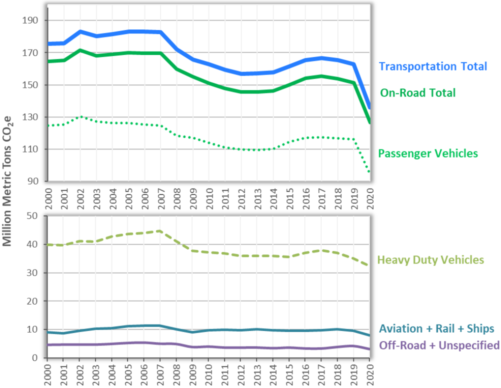
Figure 5. Overview of GHG Emissions from the Transportation Sector.
“Transportation Total” is the sum of “On-Road Total,” “Aviation + Rail + Ships,” and “Off-Road + Unspecified.” “On-
Road Total” is the sum of “Passenger Vehicles” and “Heavy Duty Vehicles.”
The fuel efficiency of the passenger vehicle fleet has generally been rising since 2009, when it was
20.3 miles per gallon (mpg), to 24.1 mpg in 2020. New 2020 model year passenger vehicles are 14
percent more fuel efficient than 2012 model year vehicles [12]. In addition, there were 336,000
battery electric vehicles (BEV) in the State in 2020, representing an 18 percent growth from 2019
[13]. Figure 6 shows the transformation of California’s light-duty fleet, with significant strides
being made in fuel efficiency improvements and zero-emission vehicle adoption.
11

Figure 6. Light Duty Vehicle Fleet Transformation.
This figure shows the fuel economy of California’s light-duty fleet and the growth in battery electric vehicles. “Gasoline
Light Duty Vehicle Fuel Economy” is the average mpg for all gasoline passenger cars, trucks, and SUVs in California.
“BEV Population” includes vehicles that do not carry any fuel (e.g., gasoline and hydrogen) or any other energy
onboard [13].
Biofuels, such as ethanol, biodiesel, and renewable diesel displace fossil fuels and reduce the
amount of fossil-based CO
2
emissions released into the atmosphere. The percentages of biodiesel
and renewable diesel in the total diesel blend
h
have shown significant growth in recent years,
growing from 0.4 percent in 2011 to 20.8 percent in 2020, due mostly to the implementation of
the Low Carbon Fuel Standard. Without biofuels, California tailpipe fossil CO
2
would be 15 MMT
higher in 2020.
Figures 7a and 7b show the trends in emissions and fuel used in light-duty gasoline and heavy-
duty diesel vehicles, respectively. Total fuel combustion emissions, inclusive of both fossil
component (orange line) and bio-component (yellow shaded region) of the fuel blend, track
trends in fuel sales. Consistent with the IPCC Guidelines for National GHG Inventory (“the IPCC
Guidelines”) [3] and the annual GHG inventories submitted by the U.S. and other nations to the
United Nations Framework Convention on Climate Change (UNFCCC), CO
2
emissions from biofuels
h
For the purpose of this report, the term “fuel blend” refers to combined, aggregated volume of fossil fuels and
biofuels that have been distributed across the state, some may be distributed as a blend of fossil fuel and biofuel while
some may be sold as biofuel. “Gasoline blend” refers to E85 and typical gasoline-ethanol fuel. ”Diesel blend” refers to
aggregation of R99, B5, pure fossil diesel, and others.
12
(the biofuel components of fuel blends) are classified as “biogenic CO
2
.” They are tracked
separately from the rest of the emissions in the inventory and are not included in the total
emissions when comparing to California’s 2020 and 2030 GHG Limits. Biogenic CO
2
emissions data
are available on California Air Resources Board (CARB) webpage [8]. Emissions of methane (CH
4
)
and nitrous oxide (N
2
O) from biofuel combustion are included in the inventory along with CO
2
,
CH
4
, and N
2
O from fossil fuel combustion.
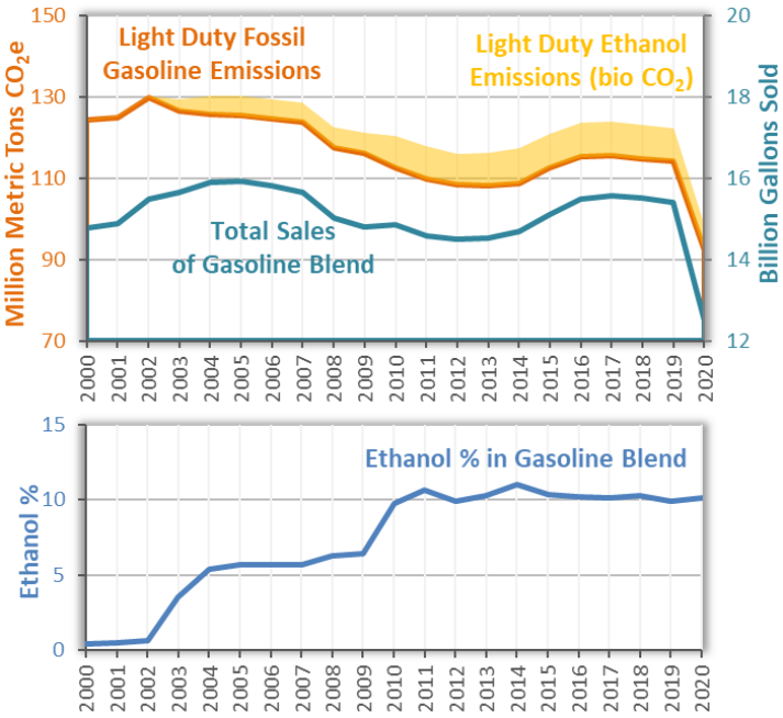
Figure 7a. Trends in On-Road Light Duty Gasoline Emissions.
In the top panel, the yellow shaded region represents CO
2
emissions from the ethanol component of the gasoline fuel
blend. The orange line includes all GHG emissions from the fossil gasoline component of the fuel blend, as well as the
CH
4
and N
2
O emissions from the ethanol component of the fuel blend. "Total Sales of Gasoline Blend" includes gasoline
used in any type of vehicle, 93% of which are used in light duty vehicles. The color of a trend line matches the color of
its corresponding vertical axis label. The bottom panel shows the percent of gasoline blend that is ethanol.
13

Figure 7b. Trends in On-Road Diesel Vehicle Emissions.
In the top panel, the yellow shaded region represents CO
2
emissions from the bio-component (biodiesel and
renewable diesel) of the diesel fuel blend. The orange line includes all GHG emissions from the fossil diesel component
of the fuel blend, as well as the CH
4
and N
2
O emissions from the bio-component of the fuel blend. "Total Sales of On-
Road Diesel" includes diesel blends used in any type of vehicle, 98% of which are used in heavy duty vehicles. The
color of a trend line matches the color of its corresponding vertical axis label. The bottom panel shows the percent of
diesel blend that are biodiesel or renewable diesel.
Electricity
Emissions from the electricity sector comprise 16 percent of 2020 statewide GHG emissions. The
GHG Inventory divides the electricity sector into two broad categories: emissions from in-state
generation (including the portion of industrial and commercial cogeneration emissions attributed
to electricity generation) and emissions from imported electricity. In-state emissions are primarily
driven by fossil gas combustion such that years with low hydropower availability typically lead to
increased emissions, as more fossil gas is required to fulfill the remaining demand. Increased
production of zero-GHG resources such as solar and wind in California and imports from other
western states also reduces demands for in-state fossil gas generation over time.
Since the early 2000’s, the deployment of renewable and less carbon-intensive resources have
facilitated the continuing decline in fossil fuel electricity generation. The Renewable Portfolio
Standard (RPS) Program and the Cap-and-Trade Program continue to incentivize the dispatch of
14

renewables over fossil fuel generation to serve California load. Higher energy efficiency standards
also counter the growth in electricity consumption that is driven by a growing population and
economy. While year-to-year fluctuations in hydropower availability result in small changes to
GHG intensity, the overall downward trend prevails for GHG intensity from electricity generation.
According to the California Energy Commission, the 2020 COVID pandemic did not have a
significant impact on total electricity consumption [15]. Figure 8 shows California’s electricity
emissions. Figure 9 shows GHG intensities of electricity generation for in-state, imports, and
overall (combining in-state and imports).
Figure 8. GHG Emissions from the Electricity Sector.
This figure shows trends in emissions of in-state electricity generation, emissions associated with electricity imported
from outside of California, and the total electricity sector emissions, which is the sum of in-state generation and
imports.
15

Figure 9. GHG Intensity of Electricity.
This figure shows trends in GHG intensities of electricity generated by in-state power plants, electricity imported from
outside of California, and the overall GHG intensities aggregating both in-state generation and electricity imports
i
.
Two overall GHG intensity metrics are presented in this figure: “Overall (consumption-based)” incorporates the
inefficiency introduced by line losses during electricity transmission and distribution, while “Overall (generation-
based)” represents state-wide average intensity at power plants before line losses are considered.
Total electric power emissions decreased in 2020 as California continued the trend of importing a
larger share of low-GHG electricity. In 2020, 45 percent of total electricity generation (in-state
generation plus imported electricity) came from solar, wind, hydropower, and nuclear power;
i
All four GHG intensities account for renewables and exclude biogenic CO
2
emissions. For calculating in-state and
overall intensities, in-state electricity emissions and generation (MWh) include on-site generation for on-site use,
cogeneration emissions attributed to electricity generation, in-state generated electricity exported out of state, and
rooftop solar. The denominator of the “overall (consumption-based)” intensity is the total electricity (MWh)
consumed in and exported from California and excludes electricity (MWh) lost during transmission and distribution in
the calculation. The denominator of the “overall (generation-based)” intensity is the total electricity generated in and
exported from California, but in this case, includes line losses in the calculation. The numerator of both consumption-
based and generation-based intensities are the total emissions from the electricity sector.
16

another six percent came from Asset Controlling Suppliers (ACS)
j
, which imported low GHG
intensity electricity consisting primarily of hydropower.
In-state solar generation grew 10 percent in 2020 compared to 2019. Between 2011 and 2020, in-
state solar generation saw significant growth as rooftop photovoltaic solar generation increased
by a factor of 11 [16] and total in-state solar generation (commercial-scale plus rooftop solar)
increased by a factor of 19 during that period [16][17]. In-state wind energy generation ramped
up through 2013 and has remained relatively constant since 2013 [17]. Figure 10 shows trends in
in-state hydro, solar, and wind electricity generation.
Figure 10. In-State Hydro, Solar, and Wind Electricity Generation.
This figure shows the amounts of electricity generated by California’s in-state wind power projects, large commercial-
scale solar power projects, rooftop solar panels, and hydropower generation stations. The units are in terawatt-hour
(1 TWh = 10
9
kWh).
j
“Asset Controlling Suppliers” are as defined by the Mandatory GHG Reporting Regulation (MRR). The term refers to
an electric power entity that owns or operates inter-connected electricity generating facilities or serves as an
exclusive marketer for these facilities even though it does not own them. Imports from ACS are primarily hydropower
but include some non-zero GHG power sources such as fossil gas.
17

Trends in the types of in-state generation are presented in Figure 11. In-state fossil gas generation
corresponds with the year-to-year fluctuations in hydro, solar, wind, and nuclear power, while
generation from other fuel types gradually decline over time.
Figure 11. In-State Electricity Generation by Fuel Type.
This figure shows the amounts of electricity generated by in-state fossil gas power plants, hydro/solar/wind/nuclear
resources, and other generation sources. The units are in terawatt-hour (1 TWh = 10
9
kWh)
k
.
k
“Other Fuels” include energy generation from associated gas, biomass, coal, crude oil, digester gas, distillate,
geothermal, jet fuel, kerosene, landfill gas, lignite coal, municipal solid waste (MSW), petroleum coke, propane,
purchased steam, refinery gas, residual fuel oil, sub-bituminous coal, synthetic coal, tires, waste coal, waste heat, and
waste oil. CO
2
and CH
4
emissions from geothermal power and CH
4
and N
2
O emissions from biomass power are
included in the statewide total for comparing to the 2020 GHG Limit. Except for geothermal power, most of these fuels
are combusted in industrial cogeneration facilities.
18

Industrial
Emissions from the industrial sector contributed 20 percent of California’s total GHG emissions
in 2020. Emissions in this sector are primarily driven by fuel combustion from sources that
include refineries, oil and gas production, cement plants, and the portion of cogeneration
emissions attributed to thermal energy output. Process emissions, such as from clinker production
in cement plants and hydrogen production for refinery use, also contribute significantly to the
total emissions for this sector. Refineries and hydrogen production represent the largest
individual source in the industrial sector, contributing 35 percent of the sector’s total emissions.
In 2020, refining and hydrogen production sector emissions decreased by 3 MMTCO
2
e (10
percent), oil and gas production emissions decreased by 2 MMTCO
2
e (13 percent), and fuel
combustion in other industrial subsectors decreased by 2 MMTCO
2
e (8 percent), leading to a
decline in 2020 industrial sector emissions of 7 MMTCO
2
e or 9 percent. Figure 12 shows emissions
trends of the industrial sector over time.
Figure 12. Industrial Sector Emissions.
The top panel of this figure shows the overall emissions trend of the total industrial sector. The bottom panel shows
emissions trends by sub-sector. Summing the bottom panel will equal the top panel. The “Other Fuel Use” category
includes emissions from combustion of fuels used by sectors not specifically broken out elsewhere in this figure. The
“Other” category includes all emissions from industrial processes and activities not belonging to a specified category
already shown in the graph. For example, leaks from fossil gas transmission and distribution infrastructure are
included in the “Oil & Gas” category. The “Cogen (thermal)” category under the industrial sector includes only the
portion of cogeneration emissions attributed to thermal output. The portion of cogeneration emissions attributed to
electricity generation is assigned to the electricity sector and not shown in this graph.
19

Commercial and Residential
Greenhouse gas emissions from the commercial and residential sectors come predominantly from
the combustion of fossil gas and other fuels for household and commercial business use, such as
space heating, cooking, water heating, and steam generation. Emissions from this sector also
include commercial and residential fertilizer application and behind-the-meter gas leaks.
l
Emissions from electricity used for cooling (air-conditioning) and appliance operation are
accounted for in the electricity sector. Emissions from refrigerants used in commercial and
residential buildings are included in the high-GWP gases category. Changes in annual fuel
combustion emissions are primarily driven by variability in weather conditions and the need for
heating in buildings, as well as population growth.
In 2020, residential and commercial sector emissions decreased by 1.7 MMTCO
2
e or 4 percent
compared to 2019 due to less need for residential space heating in winter and a reduction in
commercial fossil gas use likely due in part to the effects of the pandemic. Figure 13 presents
emissions from the commercial and residential sectors, along with heating degree days, and an
estimate of the heating energy need each year.
Figure 13. Emissions from Residential and Commercial Sectors.
Emissions from the residential and commercial sectors are compared with heating degree days, an estimate of the
heating energy need each year.
l
“Behind-the-meter” emissions include natural gas leaks after the gas passes through building-level gas meter.
Potential leak points include valves and joints of gas pipes and gas appliances. Leaks from natural gas transmission
and distribution infrastructure are accounted for in the industrial sector.
20

Emissions from fuel use by the commercial sector have seen relatively small changes from year to
year despite growth of commercial floor space by 31 percent since 2000 [19]. As a result, the
commercial sector exhibits a slight decline in fuel use per unit space due to building efficiency
increases. The number of occupied residential housing units grew steadily from 11.9 million units
in 2000 to 13.2 million units in 2020 [19]. Emissions per housing unit generally fluctuate with the
need for heating depending on the winter temperatures of the given year, which is also illustrated
by the heating degree day index in Figure 13 [21]. Figures 14 and 15 show emissions from these
sectors and the related indicators.
Figure 14. Emissions per Unit Floor Space.
This figure shows total square feet of commercial floor space and the emissions per square feet of commercial floor
space. Only fuel combustion emissions are included in the figure.
Figure 15. Emissions per Residential Housing Unit.
This figure shows number of occupied residential housing units and emissions per housing unit. Only fuel combustion
emissions are included in the figure.
21
Agriculture
California’s agricultural sector contributed 8.6 percent of statewide GHG emissions in 2020,
mainly from CH
4
and N
2
O sources. Major emissions sources in the agricultural sector include
enteric fermentation and manure management from livestock, crop production (fertilizer use, soil
preparation and disturbance, and crop residue burning), and fuel combustion associated with
agricultural activities (water pumping, cooling or heating buildings, processing commodities, and
tractors).
Approximately 71 percent of agricultural sector GHGs are emitted from livestock. Livestock
emissions in 2020 are 18 percent higher than 2000 levels. Livestock emissions are almost entirely
CH
4
generated from enteric fermentation and manure management, and most of the livestock
emissions are from dairy operations. Dairy population followed a generally increasing trend
between 2000 and 2012, and GHG emissions from dairy manure management and enteric
fermentation followed a similar trend as dairy herd sizes grew over this time. After 2012,
methane emissions from dairy operations in California have declined in proportion to population
decreases.
Crop production accounted for 21 percent of agriculture emissions in 2020. Emissions from the
growing and harvesting of crops have generally declined since 2000. The long-term trend of
emissions reduction from 2000 to 2020 corresponds to a reduction in crop acreage [22] and a
shift away from flood irrigation to sprinkler and drip irrigation. Figure 16 presents emissions
from the livestock and crop production sectors.
22

Figure 16. Agricultural Emissions.
This figure presents the trends in emissions from livestock manure management and enteric fermentation, crop
growing and harvesting (which include fertilizer application, soil preparation and disturbances, and crop residue
burning), as well as fuel combustion associated with agricultural activities (water pumping, cooling or heating
buildings, processing commodities, and tractors).
23
High Global Warming Potential Gases
In 2020, AB 32 High Global Warming Potential (high-GWP) gases comprised 5.8 percent of
California’s emissions. The GHG Inventory tracks high-GWP gas emissions from releases of ozone
depleting substance (ODS) substitutes, sulfur hexafluoride (SF
6
) emissions from the electricity
transmission and distribution system, and gases that are emitted in semiconductor manufacturing
processes. (ODSs are also high-GWP gases but are outside the scope of the IPCC accounting
framework and AB 32.) Of these tracked categories, 98 percent of high-GWP gas emissions in
2020 are ODS substitutes, which are primarily hydrofluorocarbons (HFCs). ODS substitutes are
used in refrigeration and air conditioning equipment, solvent cleaning, foam production, fire
retardants, and aerosols. In 2020, refrigeration and air conditioning equipment contributed 92
percent of ODS substitutes emissions.
Emissions of ODS substitutes have grown as these gases replace ODSs being phased out under the
Montreal Protocol [5]. Emissions of ODSs have decreased significantly since they began to be
phased out in the 1990s and dropped below ODS substitute emissions for the first time in 2015.
ODS emissions continued to drop in 2020. The combined emissions of ODS and ODS substitutes
have been steadily decreasing over time as ODSs are phased out, even as emissions from ODS
substitutes continue to increase.
Of the four main sub-sectors within the ODS substitutes category (Transportation, Commercial,
Industrial, and Residential), only the Transportation Sector has seen an emissions decrease.
Emissions from the transportation sub-sector decreased for two main reasons. The transportation
refrigeration units (TRU) Airborne Toxic Control Measure (ATCM), adopted in 2004 and
implemented in January 2010, reduces emissions by limiting the charge size of TRUs, thus
reducing leakage rates [23]. In addition, the Low-Emission Vehicle (LEV) III regulations (as part of
the Advanced Clean Cars rulemaking package) were adopted in 2012 and include increasingly
stringent emission standards for new passenger vehicles through the 2025 model year. LEV III
prescribe measures that lower refrigerant emissions, including reducing end-of-life losses for
passenger vehicle air conditioning systems. Figures 17a and 17b show ODS substitutes’ emissions.
24

Figure 17a. Trends in ODS and ODS Substitutes Emissions.
This figure presents the trends in emissions from ODS substitutes, ODS, and their sum (“Total Emissions”). ODS
substitutes emissions are specified in the IPCC Guidelines and AB 32 and are included in the GHG Inventory. ODSs are
also GHGs but are tracked separately outside of the GHG Inventory.
Figure 17b. ODS Substitutes Emissions by Category.
This figure presents the breakdown of ODS substitutes emissions by product type and sector category in 2020.
Refrigerants used in various sectors make up the majority of ODS substitutes emissions.
25

Recycling and Waste
Emissions from the recycling and waste sector include CH
4
and N
2
O emissions from landfills and
from commercial-scale composting. Emissions from recycling and waste, which comprise
two percent of California’s GHG Inventory, have grown by 25 percent since 2000. Landfill
emissions are primarily CH
4
and account for 96 percent of the emissions from this sector in 2020,
while compost production facilities make up the remaining fraction of emissions.
The emissions from a landfill are the difference between the methane generated from waste
decomposition and the methane captured by landfill gas collection and control system. The annual
amount of solid waste deposited in California’s landfills grew from 39 million short tons in 2000 to
its peak of 46 million short tons in 2005, followed by a declining trend until 2012. After 2012,
deposited waste amounts have seen a steady rise over time, with the exception of a drop in 2020
likely due in part to the COVID19 pandemic and the resulting decline in commercial and industrial
waste generation [24]. Landfill methane generation is driven by the total amount of degradable
carbon remaining in California landfills, rather than year-to-year fluctuation in annual deposition
of solid waste [25]. Figures 18 and 19 show trends in landfill emissions and activities that drive
emissions.
Figure 18. Landfill Methane Emissions.
This figure presents trends in landfill emissions and the amount of degradable carbon remaining in California landfills.
The latter drives the emissions generated by landfills. The color of a trend line matches the color of its corresponding
vertical axis label.
26

Figure 19. Landfill Waste.
The top panel presents the annual amounts of solid waste deposited into California landfills and the amount of
degradable carbon contained in the solid waste. The color of a trend line matches the color of its corresponding
vertical axes label. The bottom panel shows estimated amounts of compost feedstock processed by the state’s
composting facilities.
27
Additional Information
International GHG Inventory Practice of Recalculating Emissions for
Previous Years
Consistent with the IPCC GHG inventory guidelines, recalculations are made to incorporate new
methods or reflect updated data for all years from 2000 to 2019 to maintain a consistent
inventory time series. Therefore, emission estimates for a given calendar year may be different
between editions as methods and supplemental data are updated. For example, in the 2021
edition, total 2019 emissions were estimated to be 418.2 MMTCO
2
e. In the 2022 edition,
recalculation revised the 2019 emissions to 404.5 MMTCO
2
e, reflecting refinements and updates
to methodology and information gained since 2021. Analyses of emission trends, including the
emissions decrease of 35.3 MMTCO
2
e between 2019 and 2020, are based on the recalculated
numbers in the 2022 edition of the inventory. A description of the method updates can be found
here: https://ww2.arb.ca.gov/sites/default/files/classic/cc/inventory/
ghg_inventory_00-20_method_update_document.pdf
Global Warming Potential Values
In accordance with the IPCC GHG inventory guidelines, California’s GHG Inventory uses the 100-
year GWPs from the IPCC 4th Assessment Report, consistent with the national GHG inventories
submitted by the U.S. and other nations to the UNFCCC. However, other CARB programs may use
different GWP values. For example, the SLCP Reduction Strategy [4] uses a 20-year GWP because
the SLCP has greater climate impact in the near-term compared to the longer-lived GHGs, such as
CO
2
.
Sources of Data Used in the GHG Emission Inventory
Statewide GHG emissions are calculated using several data sources. The primary data source is
from reports submitted to the California Air Resources Board (CARB) through the Regulation for
the Mandatory Reporting of GHG Emissions (MRR). MRR requires facilities and entities with more
than 10,000 metric tons CO
2
e per year of combustion and process emissions, all facilities
belonging to certain industries, and all electricity importers to submit an annual GHG emissions
data report directly to CARB. Reports from facilities and entities that emit more than 25,000
metric tons of CO
2
e per year are verified by a CARB-accredited third-party verification body.
Starting with the 2022 edition of the GHG Emission Inventory, the methodology for the inventory
was updated to more clearly reflect MRR emissions data. More information on MRR emissions
reports can be found at: https://ww2.arb.ca.gov/mrr-data
CARB also relies on data from other California State and federal agencies to develop the annual
statewide GHG emission inventory for the State of California. These additional sources include,
but are not limited to, data from the California Energy Commission, California Department of Tax
and Fee Administration, California Geologic Energy Management Division, California Department
of Food and Agriculture, CalRecycle, U.S. Energy Information Administration, and U.S.
Environmental
28
Protection Agency (U.S. EPA). The timing for when these data sources are available drives the
publication date for the inventory each year. All data sources used to develop the GHG Inventory
are listed in the GHG emission inventory supporting documentation at:
https://ww2.arb.ca.gov/ghg-inventory-data.
The main GHG Inventory page is located at:
https://ww2.arb.ca.gov/our-work/programs/ghg-inventory-program.
Other Ways of Categorizing Emissions in the Inventory
There is more than one way of organizing emissions by category in an inventory. Each year,
CARB makes the GHG Inventory available in three categorization schemes:
• The Scoping Plan Categorization organizes emissions by CARB program structure. (This is
the categorization scheme used in this report.)
• The Economic Sector/Activity Categorization generally aligns with how sectors are defined
in the North America Industry Classification System (NAICS).
• The IPCC Categorization groups emissions into four broad categories of emission
processes. This format conforms to international GHG inventory practice and is consistent
with the national GHG inventory that U.S. EPA annually submits to the United Nations.
Although this report uses the Scoping Plan Categorization in the presentation and discussion of
emissions, the Economic Sector/Activity Categorization is also often used by the public. The
difference between the Scoping Plan Categorization and the Economic Sector/Activity
Categorization are as follows: (1) High-GWP gases are shown as its own category under the
Scoping Plan categorization, but under the economic sector categorization, they are included as
part of the economic sectors where they are used. (2) The recycling and waste sector is shown as
its own category under the Scoping Plan categorization but is included as part of the industrial
sector under the Economic Sector/Activity Categorization.
The figures below show the Scoping Plan Categorization and the Economic Sector/Activity
Categorization side-by-side. Detailed data for these categorization schemes can be accessed from
CARB webpage at: https://ww2.arb.ca.gov/ghg-inventory-data.
29

Figure 20a. 2020 GHG Emissions by Economic Sector.
This figure shows the relative size of 2020 emissions by economic sector.
Figure 20b. 2020 GHG Emissions by Scoping Plan Category*.
This figure shows the relative size of 2020 emissions, organized by the categories in the AB 32 Scoping Plan. *Due to
rounding, numbers may not add up to 100%.
30
Uncertainties in the Inventory
CARB is committed to continually working to reduce the uncertainty in the inventory estimates.
The uncertainty of emissions estimates in the inventory varies by sector. The emissions data
reported under MRR is subject to third-party verification, ensuring a high level of accuracy. Other
non-MRR sources, mainly non-combustion, biochemical processes, have varying uncertainty
depending on the input data and the emission processes.
Natural and Working Lands Ecosystem Carbon Inventory and Wildfire
Emissions
CARB has also developed a Natural and Working Lands (NWL) Ecosystem Carbon Inventory [2]
(“the NWL Inventory”) separate from this GHG Inventory. The NWL Inventory quantifies
ecosystem carbon stored in plants and soils in California’s Natural and Working Lands (including
forest, woodland, shrubland, grassland, wetland, orchard crop, urban forest, and soils) and tracks
changes in carbon stock over time. The NWL Inventory report can be accessed here:
https://ww2.arb.ca.gov/nwl-inventory.
Fire has served a natural function in California's diverse ecosystems for millennia, such as
facilitating germination of seeds for certain tree species, replenishing soil nutrients, clearing dead
biomass to make room for living trees to grow, and reducing accumulation of fuel that lead to
high-intensity wildfires. Fire also impacts human health and safety, and releases GHGs and other
air pollutants. Greenhouse gas emissions from wildfires are tracked separately when compared to
anthropogenic sources due to carbon cycling. Anthropogenic emissions from fossil fuels come
from geological sources, which are part of the slow carbon cycle, where carbon pools change over
the course of many millennia (e.g., fossil fuel formation). In contrast, the fast carbon cycle, in
which carbon moves between pools over months to centuries, includes natural emission sources,
such as wildfires, plant decomposition and respiration. The acceleration of fossil fuel burning has
led to an increase in ambient CO
2
concentrations; however, wildfire emissions are part of a fast
carbon cycle that is balanced by vegetation growth. In recent years the intensity and size of
wildfires have increased across California. In an effort to contextualize the GHG emissions from
wildfires, CARB annually publishes wildfire emissions estimates here:
https://ww2.arb.ca.gov/wildfire-emissions.
Frequently asked questions regarding wildfire emissions are available here:
https://ww3.arb.ca.gov/cc/inventory/pubs/wildfire_emissions_faq.pdf.
Pesticides
The list of GHGs to be included in the scope of the GHG Inventory is defined by AB 32 and the IPCC
Guidelines. There are pesticides that act as GHGs but are not in the list of GHGs in AB 32 nor the
IPCC Guidelines; and therefore, they are not tracked as part of the GHG Inventory. Two examples
include methyl bromide, a fumigant used to control pests in agriculture and shipping, and sulfuryl
fluoride, a pesticide used for building fumigation and post-harvest storage of commodities but not
licensed for use in agricultural fields. CARB has provided estimates of sulfuryl fluoride emissions
31

Figure References
Figure Number
Reference
Figure 1
[8]
Figure 2a
[8] [9] [10]
Figure 2b
[8] [9]
Figure 2c
[8] [10]
Figure 3
[8]
Figure 4
[8]
Figure 5
[8]
Figure 6
[11] [12] [13] [14]
Figure 7a & 7b
[8]
Figure 8
[8]
Figure 9
[8] [16] [17] [18]
Figure 10
[16] [17]
Figure 11
[16] [17]
Figure 12
[8]
Figure 13
[8] [20]
Figure 14
[8] [19]
Figure 15
[8] [20]
Figure 16
[8]
Figure 17a & 17b
[8] [23]
Figure 18
[8]
Figure 19
[8] [24] [26]
Figure 20a & 20b
[8]
33
References
[1] State of California, "California Health and Safety Code, Division 25.5, Part 1, Chapter 3,
Section 38505(g)," 2006. [Online]. Available:
https://leginfo.legislature.ca.gov/faces/billNavClient.xhtml?bill_id=200520060AB32
[2] California Air Resources Board, "An Inventory of Ecosystem Carbon in California's Natural
& Working Lands," 2018. [Online]. Available:
https://ww3.arb.ca.gov/cc/inventory/pubs/nwl_inventory.pdf
[3] Intergovernmental Panel on Climate Change, "IPCC Guidelines for National greenhouse Gas
Inventories, Volume 1 - General Guidance and Reporting," [Online]. Available:
https://www.ipcc-nggip.iges.or.jp/public/2006gl/vol1.html
[4] California Air Resources Board, "Short-Lived Climate Pollutant (SLCP) Strategy," 2017.
[Online]. Available: https://www.arb.ca.gov/cc/shortlived/shortlived.htm
[5] United Nations Environmental Programme, "Treaties and Decisions - The Montreal
Protocol on Substances that Deplete the Ozone Layer," 2015. [Online]. Available:
http://ozone.unep.org/en/treaties-and-decisions/montreal-protocol-substances-deplete-
ozone-layer
[6] California Air Resources Board, "First Update to the Climate Change Scoping Plan Building
on the Framework Pursuant to AB32: California's Global Warming solutions Act 2006,"
2014. [Online]. Available:
https://ww2.arb.ca.gov/sites/default/files/classic//cc/scopingplan/2013_update/first_updat
e_climate_change_scoping_plan.pdf
[7] Intergovernmental Panel on Climate Change, "Fourth Assessment Report," 2007. [Online].
Available: https://www.ipcc.ch/assessment-report/ar4/
[8] California Air Resources Board, "GHG Emissions Inventory (GHG EI) 2000-2020," 2022.
[Online]. Available: https://ww2.arb.ca.gov/ghg-inventory-data
[9] California Department of Finance, "E-6. Population estimates and components of change by
county 2010-2021," 2022. [Online]. Available:
https://dof.ca.gov/forecasting/demographics/estimates/estimates-e6-2010-2021/
[10] California Department of Finance, "California Gross Domestic Product," 2022. [Online].
Available: https://dof.ca.gov/forecasting/economics/economic-indicators/gross-state-
product/
34
[11] CARB-MSAB Reference. California Department of Tax and Fee Administration. (2022, 08
22). Fuel Taxes Statistics & Reports. Retrieved from https://www.cdtfa.ca.gov/taxes-and-
fees/spftrpts.htm
[12] California Air Resources Board, EMFAC2021. 2022. [Online]. Available:
https://arb.ca.gov/emfac/
[13] EMFAC Fleet Database. (2022). Emission Factors Model – Fleet Database. [Online].
Available: https://arb.ca.gov/emfac/fleet-db
[14] USEPA. (2022) U.S. Environmental Protection Agency – Fuel Economy Guide. [Online].
Available: www.fueleconomy.gov
[15] California Energy Commission (a). 2022. California Energy Consumption Database.
Available: http://www.ecdms.energy.ca.gov/Default.aspx
[16] California Energy Commission (b). 2022. Gautam, A, Personal Communication Between the
California Air Resources Board (L. Hunsaker) and the California Energy Commission (A.
Gautam), 2022
[17] U.S. Energy Information Administration, "Electricity - Form EIA-923 Detailed Data with
Previous Form Data (EIA-906/920)," 2022. [Online]. Available:
https://www.eia.gov/electricity/data/eia923/
[18] California Air Resources Board, "Summary of 2008 to 2020 Data from California's
Greenhouse Gas Mandatory Reporting Program," 2022. [Online]. Available:
https://ww2.arb.ca.gov/mrr-data
[19] California Energy Commission (c). 2022. Vaid, R, Personal Communication Between the
California Air Resources Board (B. Widger) and the California Energy Commission (R.
Vaid), 2022
[20] State of California, Department of Finance, E-5 Population and Housing Estimates for Cities,
Counties and the State — January 1, 2011-2020. Sacramento, California, 2022. [Online].
Available: https://dof.ca.gov/forecasting/demographics/estimates/estimates-e5-2010-2020/
[21] National Oceanic and Atmospheric Administration, "Heating and Cooling Degree Days,"
2022. [Online]. Available:
ftp.cpc.ncep.noaa.gov/htdocs/products/analysis_monitoring/cdus/degree_days/archives/He
ating%20degree%20Days/monthly%20states/
[22] U.S. Department of Agriculture, "National Agricultural Statistics Service," 2022. [Online].
Available: https://quickstats.nass.usda.gov/
35
[23] G. Gallagher, T. Zhan, Y.-K. Hsu, P. Gupta, J. Pederson, B. Croes, D. R. Blake, B. Barletta, S.
Meindardi, P. Ashford, A. Vetter, S. Saba, R. Slim, L. Palandre, D. Clodic, P. Mathis, M.
Wagner, J. Forgie, H. Dwyer and K. Wolf, "High-Global Warming Potential F-Gas Emissions
in California: Comparison of Ambient-Based Versus Inventory-Based Emission Estimates,
and Implications of Refined Estimates," Environmental Science & Technology, pp. 1084-
1093, 21 January 2014
[24] CalRecycle, "Landfill Tonnage Reports, 2000-2020," 2022. [Online]. Available:
https://www2.calrecycle.ca.gov/LandfillTipFees/
[25] Intergovernmental Panel on Climate Change, "IPCC Guidelines for National Greenhouse Gas
Inventories, Volume 5 - Waste: IPCC Waste Model," 2006. [Online]. Available:
https://www.ipcc-nggip.iges.or.jp/public/2006gl/vol5.html
[26] CalRecycle, "Compost and Mulch Producers," 2022. [Online]. Available:
https://calrecycle.ca.gov/organics/processors/
36
