CoDa.dvi

Lecture Notes

Compositional Data Analysi s

V. Pawlowsky-Glahn

J. J. Egozcue

R. Tolosana-Delgado

2007

Prof. Dr. Vera Pawlowsky-Glahn

Catedr´atica de Universidad (Full professor)

University of Girona

Dept. of Computer Science and Applied Mathematics

Campus Montilivi — P-1, E-17071 Girona, Spain

vera.pawlo[email protected]du

Prof. Dr. Juan Jos´e Egozcue

Catedr´atico de Universidad (Full professor)

Technical University of Catalonia

Dept. of Applied Mathematics III

Campus Nord — C-2, E-08034 Barcelona, Spain

[email protected]

Dr. Raimon Tolosana-Delgado

Wissenschaft licher Mitarbeiter (fellow scientist)

Georg-August-Universit¨at G¨ottingen

Dept. of Sedimentology and Environmental Geology

Goldschmidtstr. 3, D-37077 G¨ottingen, Germany

[email protected]ettingen.de

Preface

These notes have been prepared as support to a short course on compositional data

analysis. Their aim is to transmit the basic concepts and skills for simple applications,

thus setting the premises for more advanced projects. One should be aware that frequent

updates will be required in the near future, as the theory presented here is a ﬁeld of

active research.

The notes are based both on the monograph by John Aitchison, Statistical analysis

of compositional data (1986), and on recent developments that complement the theory

developed there, mainly those by Aitchison, 1997; Barcel´o- Vidal et al., 200 1; Billheimer

et al., 2001; Pawlowsky-Glahn and Egozcue, 2001, 2002; Aitchison et al., 2002; Egozcue

et al., 2003; Pawlowsky-Glahn, 2003; Egozcue and Pawlowsky-Glahn, 2005. To avoid

constant references to mentioned documents, only complementary references will be

given within the text.

Readers should be aware that for a thoro ugh understanding of compositional data

analysis, a good knowledge in standard univariate statistics, basic linear algebra and

calculus, complemented with an introduction to applied multivariate statistical analysis,

is a must. The speciﬁc subjects of interest in multivariate statistics in real space can

be learned in parallel from standard textbooks, like for instance Krzanowski (1988)

and Krzanowski and Marriott (1994) (in English), Fahrmeir and Hamerle (1984) (in

German), or Pe˜na (2002) (in Spanish). Thus, the intended audience goes from advanced

students in applied sciences to practitioners.

Concerning notation, it is important to note that, to conform to the standard praxis

of registering samples as a matrix where each row is a sample and each column is a

variate, vectors will be considered as row vectors t o make the transfer from theoretical

concepts to practical computations easier.

Most chapters end with a list of exercises. They are formulated in such a way that

they have to be solved using an a ppropriate software. A user friendly, MS-Excel based

freeware to facilitate this task can be downloaded from the web at the following address:

http://ima.udg.edu/Recerca/EIO/inici

eng.html

Details about this package can be found in Thi´o-Henestrosa and Mart´ın-Fern´andez

(2005) or Thi´o-Henestrosa et al. (2005). There is a lso available a whole library o f

ii Preface

subroutines for Matlab, developed mainly by John Aitchison, which can be obtained

from John Aitchison himself or from anybody of the compositional data analysis group

at the University of Girona. Finally, those interested in working with R (or S-plus)

may either use the set of functions “mixeR” by Bren (2003), or the full-ﬂedged package

“compositions” by van den Boogaart and Tolosana-Delgado (2005).

Contents

Preface i

1 Introduction 1

2 Compositional data and their sample space 5

2.1 Basic concepts . . . . . . . . . . . . . . . . . . . . . . . . . . . . . . . . . 5

2.2 Principles of compositional ana lysis . . . . . . . . . . . . . . . . . . . . . 7

2.2.1 Scale invariance . . . . . . . . . . . . . . . . . . . . . . . . . . . . 7

2.2.2 Permutation invaria nce . . . . . . . . . . . . . . . . . . . . . . . . 9

2.2.3 Subcompositional coherence . . . . . . . . . . . . . . . . . . . . . 9

2.3 Exercises . . . . . . . . . . . . . . . . . . . . . . . . . . . . . . . . . . . . 10

3 The Aitchison geometry 11

3.1 General comments . . . . . . . . . . . . . . . . . . . . . . . . . . . . . . 11

3.2 Vector space structure . . . . . . . . . . . . . . . . . . . . . . . . . . . . 12

3.3 Inner product, norm and distance . . . . . . . . . . . . . . . . . . . . . . 14

3.4 Geometric ﬁgures . . . . . . . . . . . . . . . . . . . . . . . . . . . . . . . 15

3.5 Exercises . . . . . . . . . . . . . . . . . . . . . . . . . . . . . . . . . . . . 15

4 Coordinate representation 17

4.1 Introduction . . . . . . . . . . . . . . . . . . . . . . . . . . . . . . . . . . 17

4.2 Compositional observations in real space . . . . . . . . . . . . . . . . . . 18

4.3 Generating systems . . . . . . . . . . . . . . . . . . . . . . . . . . . . . . 18

4.4 Orthonormal coordinates . . . . . . . . . . . . . . . . . . . . . . . . . . . 20

4.5 Working in coordinates . . . . . . . . . . . . . . . . . . . . . . . . . . . . 25

4.6 Additive log- r atio coordinates . . . . . . . . . . . . . . . . . . . . . . . . 27

4.7 Simplicial matrix notation . . . . . . . . . . . . . . . . . . . . . . . . . . 28

4.8 Exercises . . . . . . . . . . . . . . . . . . . . . . . . . . . . . . . . . . . . 31

5 Exploratory data analysis 33

5.1 General remarks . . . . . . . . . . . . . . . . . . . . . . . . . . . . . . . . 33

5.2 Centre, total variance and variation matrix . . . . . . . . . . . . . . . . . 34

iii

iv Contents

5.3 Centring and scaling . . . . . . . . . . . . . . . . . . . . . . . . . . . . . 35

5.4 The biplot: a graphical display . . . . . . . . . . . . . . . . . . . . . . . 36

5.4.1 Construction of a biplot . . . . . . . . . . . . . . . . . . . . . . . 36

5.4.2 Interpretation of a compositional biplot . . . . . . . . . . . . . . . 38

5.5 Exploratory analysis of coordinates . . . . . . . . . . . . . . . . . . . . . 39

5.6 Illustration . . . . . . . . . . . . . . . . . . . . . . . . . . . . . . . . . . . 40

5.7 Exercises . . . . . . . . . . . . . . . . . . . . . . . . . . . . . . . . . . . . 46

6 Distributions on the simplex 49

6.1 The normal distribution on S

. . . . . . . . . . . . . . . . . . . . . . . 49

6.2 Other distributions . . . . . . . . . . . . . . . . . . . . . . . . . . . . . . 50

6.3 Tests of normality on S

. . . . . . . . . . . . . . . . . . . . . . . . . . . 50

6.3.1 Marginal univariate distributions . . . . . . . . . . . . . . . . . . 51

6.3.2 Bivariate angle distribution . . . . . . . . . . . . . . . . . . . . . 53

6.3.3 Radius test . . . . . . . . . . . . . . . . . . . . . . . . . . . . . . 54

6.4 Exercises . . . . . . . . . . . . . . . . . . . . . . . . . . . . . . . . . . . . 56

7 Statistical inference 57

7.1 Testing hypothesis a bout two groups . . . . . . . . . . . . . . . . . . . . 57

7.2 Probability and conﬁdence regions for compositional data . . . . . . . . . 60

7.3 Exercises . . . . . . . . . . . . . . . . . . . . . . . . . . . . . . . . . . . . 62

8 Compositional processes 63

8.1 Linear processes: expo nential growth or decay of mass . . . . . . . . . . 63

8.2 Complementary processes . . . . . . . . . . . . . . . . . . . . . . . . . . 66

8.3 Mixture process . . . . . . . . . . . . . . . . . . . . . . . . . . . . . . . . 70

8.4 Linear regression with compositional response . . . . . . . . . . . . . . . 72

8.5 Principal component analysis . . . . . . . . . . . . . . . . . . . . . . . . 75

References 81

Appendices a

A. Plotting a ternary diagram a

B. Parametrisation of an elliptic region c

Chapter 1

Introduction

The awareness of problems related to the statistical analysis of comp ositional data

analysis dates back to a paper by Karl Pearson (1897) which title began signiﬁcantly

with the words “On a form o f spurious correlation ... ”. Since then, as stated in

Aitchison and Egozcue (2005), the way to deal with this type of data has g one through

roughly four phases, which they describe as follows:

The pre-1960 phase rode on the crest of the developmental wave of stan-

dard multivariate statistical analysis, a n appropriate form of analysis for

the investigation of problems with real sample spaces. Despite the obvious

fact that a compositional vector—with components the proportions of some

whole—is subject to a constant-sum constraint, and so is entirely diﬀerent

from the unconstrained vector of standard unconstrained multivariate sta-

tistical analysis, scientists and statisticians alike seemed almost to delight in

applying all the intricacies of standard multivariate analysis, in particular

correlation analysis, to compositional vectors. We know that Ka r l Pearson,

in his deﬁnitive 1897 paper on spurious correlations, had pointed out the

pitfalls of interpretation of such activity, but it was not until around 1960

that speciﬁc condemnation of such an approach emerged.

In the second phase, the primary critic of the application of standard

multivariate analysis to compositional data was the geologist Felix Chayes

(1960), whose main criticism was in the interpretation of product-moment

correlation between components of a g eochemical composition, with negative

bias the distorting factor from the viewpoint o f any sensible interpretation.

For this problem of negative bias, often referred to as the closure problem,

Sarmanov and Vistelius (1959) supplemented the Chayes criticism in geolog-

ical applications and Mosimann (1962) drew the attention of biologists to it.

However, even conscious researchers, instead of working towards an appro-

priate methodology, adopted what can only be described as a pathological

2 Chapter 1. Intr oduction

approach: distortion of standard multivariat e techniques when applied to

compositional data was the main goal of study.

The third phase was the realisation by Aitchison in the 1980’s that com-

positions provide information about relative, not a bsolute, values of com-

ponents, that therefore every statement about a composition can be stated

in terms of ratios of components (Aitchison, 1981, 1982, 1983, 1984). The

facts that logra tios are easier to handle mathematically than ratios and

that a logratio transformation provides a one-to-one mapping on to a real

space led to the advocacy of a methodology based on a variety of logratio

transformations. These transformations allowed the use of standard uncon-

strained multivariate statistics applied to transformed data, with inferences

translatable back into compositional statements.

The fourth phase arises from the realisation t hat the internal simpli-

cial operation of perturbation, the external operation of powering, and the

simplicial metric, deﬁne a metric vector space (indeed a Hilbert space) (Bill-

heimer et al. 1997, 2001; Pawlowsky-Glahn and Egozcue, 2001). So, many

compositional problems can be investigated within this space with its spe-

ciﬁc algebraic-geometric structure. There has thus arisen a staying-in-the-

simplex approach to the solution of many compositional problems (Mateu-

Figueras, 2003; Pawlowsky-Glahn, 2003 ). This staying-in-the-simplex point

of view proposes to represent compositions by their coordinates, as they live

in an Euclidean space, and to interpret them and their relationships from

their representation in the simplex. Accordingly, the sample space of ran-

dom compositions is identiﬁed to be the simplex with a simplicial metric and

measure, diﬀerent from the usual Euclidean metric and Lebesgue measure

in real space.

The third phase, which mainly deals with (log-ratio) transformation of

raw data, deserves special attention because these techniques have been very

popular and successful over more than a century; from the Galton-McAlister

introduction of such an idea in 1879 in their logarithmic transformation for

positive dat a, through variance-stabilising transformations for sound analy-

sis of variance, to the general Box-Cox transformation (Box and Cox, 19 64)

and the implied transformations in generalised linear modelling. The logra-

tio transformation principle was based on the fact that there is a one-to-one

correspondence between compositional vectors and associated logratio vec-

tors, so that any statement about compositions can be reformulated in terms

of logratios, and vice versa. The advantag e of the transformation is that it

removes the problem of a constrained sample space, the unit simplex, to one

of an unconstrained space, multivariate real space, opening up all available

standard multivariate techniques. The original transformations were princi-

pally the additive logratio transformation (Aitchison, 1986, p.113) and the

centred logratio transformation (Aitchison, 1986, p.79). The logratio trans-

formation methodology seemed to be accepted by the statistical community;

see for example the discussion of Aitchison (1982). The logratio method-

ology, however, drew ﬁerce o pposition f r om other disciplines, in particular

from sections of the geological community. The reader who is interested in

following the arg uments that have arisen should examine the Letters to the

Editor of Mathematical Geology over the period 1988 through 2 002.

The notes presented here correspond to the fourth phase. They pretend to sum-

marise the state-of-the-art in the staying-in-the-simplex approach. Therefore, the ﬁrst

part will be devoted to the algebraic-geometric structure of the simplex, which we call

Aitchison geometry.

4 Chapter 1. Intr oduction

Chapter 2

Compositional data and their

sample space

2.1 Basic concep ts

Deﬁnition 2.1. A row vector, x = [x

, x

, . . . , x

], is deﬁned as a D-part composition

when all its components are strictly positive real numbers and they carry only relative

information.

Indeed, that compositional information is relative is implicitly stated in the units, as

they ar e always parts of a whole, like weight or volume percent, ppm, ppb, or molar

proportions. The most common examples have a constant sum κ and are known in the

geological literature as closed data (Chayes, 1971 ). Frequently, κ = 1, which means

that measurements have been made in, or transformed to, parts per unit, or κ = 100,

for measurements in percent. Other units are possible, like ppm or ppb, which are

typical examples for compositional data where only a part of the composition has been

recorded; or, as recent studies have shown, even concentration units (mg/L, meq/L,

molarities and molalities), where no constant sum can be feasibly deﬁned (Buccianti

and Pawlowsky-Glahn, 2005; Otero et al., 2005).

Deﬁnition 2.2. The sample space of compositional data is the simplex, deﬁned as

= {x = [x

, x

, . . . , x

] |x

> 0, i = 1, 2, . . . , D;

i=1

= κ}. (2.1)

However, this deﬁnition does not include compositions in e.g. meq/L. Therefore, a more

general deﬁnition, together with its interpretation, is given in Section 2.2.

Deﬁnition 2.3. For any vector of D real positive components

z = [z

, z

, . . . , z

] ∈ R

6 Chapter 2. Sample space

Figure 2.1: Left: Simplex imbedded in R

. Right: Ternary diagram.

> 0 for a ll i = 1, 2, . . . , D), the closure of z is deﬁnd as

C(z) =

κ · z

i=1

κ · z

i=1

, ··· ,

κ · z

i=1

The result is the same vector rescaled so that the sum of its components is κ. This

operation is required for a formal deﬁnition of subcomposition. No te that κ depends

on the units of measurement: usual values are 1 (proportions), 100 (%), 10

(ppm) and

(ppb).

Deﬁnition 2.4. Given a composition x, a subcomposition x

with s parts is obtained

applying the closure operation to a subvector [x

, x

, . . . , x

] of x. Subindexes i

, . . . , i

tell us which parts are selected in the subcomposition, not necessarily the ﬁrst s ones.

Very often, compositions contain many variables; e.g., the major oxide bulk compo-

sition of igneous rocks have around 10 elements, and they are but a few of the total

possible. Nevertheless, one seldom represents the full sample. In fact, most of the

applied literature on compositional data analysis (mainly in geology) restrict their ﬁg-

ures to 3 -part (sub)compositions. For 3 parts, the simplex is an equilateral triangle, as

the one represented in Figure 2.1 left, with vertices at A = [κ, 0, 0], B = [0, κ, 0] and

C = [0, 0, κ]. But t his is commonly visualized in the fo r m of a ternary diagram—which

is an equiva lent representation—. A ternary diagram is an equilateral triangle such

that a generic sample p = [p

, p

] will plot at a distance p

from the opposite side

of vertex A, at a distance p

from the opposite side of vertex B, and at a distance p

from the opposite side of vertex C, as shown in Figure 2.1 right. The triplet [p

, p

]

is commonly called the barycentric coordinates of p, easily interpretable but useless in

plotting (plotting them would yield the three-dimensional left-hand plot o f Figure 2.1).

What is needed (to get the right-hand plot of the same ﬁgure) is the expression of the

2.2 Principles of compositional analysis 7

coordinates of the vertices and o f the samples in a 2-dimensional Cartesian co ordinate

system [u, v], and this is given in Appendix A.

Finally, if only some parts of the composition are available, we may either deﬁne

a ﬁll up or residual value, or simply close the observed subcomposition. Note that,

since we almost never analyse every possible part, in fact we are always working with

a subcomposition: the subcomposition of analysed parts. In any case, both methods

(ﬁll-up or closure) should lead to identical results.

2.2 Principles of compositional analysis

Three conditions should be fulﬁlled by any statistical method to be applied to com-

positions: scale invariance, permutation invariance, and subcompositional coherence

(Aitchison, 1986).

2.2.1 Scale invariance

The most important characteristic of compositional data is that they carry onl y relative

information. Let us explain this concept with an example. In a paper with the sugges-

tive title of “unexpected trend in the compositional maturity of second-cycle sands”,

Solano-Acosta and Dutta (2005) analysed the lithologic composition of a sandstone and

of its derived recent sands, looking at the percentage of grains made up o f only quartz,

of only feldspar, or of rock f r agments. For medium sized grains coming from the parent

sandstone, they report an average composition [Q, F, R] = [53, 41, 6] %, whereas for the

daughter sands the mean values are [37, 53, 10] %. One expects that feldspar and rock

fragments decrease as the sediment matures, thus they should be less important in a

second generation sand. “Unexpectedly” (or apparently), this does not happen in their

example. To pass from the parent sandstone to t he daughter sand, we may think of

several diﬀerent changes, yielding exactly the same ﬁnal composition. Assume those

values were weight percent (in gr/100 gr of bulk sediment). Then, one of the following

might have happened:

• Q suﬀered no change passing from sandstone t o sand, but 35 gr F and 8 gr R were

added to the sand (for instance, due to comminution o f coarser grains of F and R

from the sandstone),

• F was unchanged, but 25 gr Q were depleted from the sandstone and at the same

time 2 gr R were added (for instance, because Q was better cemented in the

sandstone, thus it tends to form coarser grains),

• any combination of the former two extremes.

8 Chapter 2. Sample space

The ﬁrst two cases yield ﬁnal masses of [53, 76, 14] gr, resp ectively [28, 41, 8] gr. In a

purely compositional data set, we do not know if we added or subtracted mass from

the sandstone to the sand. Thus, we cannot decide which of these cases really oc-

curred. Without further (non-compositional) information, there is no way to distin-

guish between [5 3, 76, 14] gr and [28, 41, 8] gr, as we only have the value of the sand

composition after closure. Closure is a projection of any p oint in the positive orthant

of D-dimensional real space onto the simplex. All points on a ray starting at the

origin (e. g . , [53, 76, 14] and [28, 41, 8 ]) are projected onto the same point of S

(e.g.,

[37, 53, 10] %). We say that the ray is an equivalence class and the point on S

a rep-

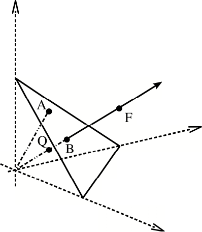
resentant of the class: Figure 2.2 shows this relationship. Moreover, if we change the

Figure 2 .2 : Repr e sentation of the compositional equivalence relationship. A represents the original

sandstone composition, B the ﬁnal sand comp osition, F the amount of each part if feldspar was added

to the system (ﬁrst hyp othesis), and Q the amount of each part if quartz was depleted from the system

(second hypothesis). Note that the po ints B, Q and F are compositionally equivalent.

units of our data (for instance, from % to ppm), we simply multiply all our points by

the constant of change of units, moving them along their rays to t he intersections with

another triangle, parallel to the plotted one.

Deﬁnition 2.5. Two vectors of D positive real compo nents x, y ∈ R

, y

≥ 0 for all

i = 1, 2, . . . , D), are com positionally equivalent if there exists a positive scalar λ ∈ R

such that x = λ · y and, equivalently, C(x) = C(y).

It is highly reasonable t o ask our analyses to yield the same result, independently of

the value of λ. This is what Aitchison (1986) called scale invariance:

2.3 Exercises 9

Deﬁnition 2.6. a function f(·) is scale-invariant if for any p ositive real value λ ∈ R

and for any composition x ∈ S

, the function satisﬁes f (λx) = f(x), i.e. it yields the

same result for a ll vectors compositionally equivalent.

This can only be achieved if f(·) is a function only of log-ratios of the parts in x

(equivalently, of r atios of parts) (Aitchison, 1997; Barcel´o-Vidal et al., 2001).

2.2.2 Permutation invariance

A function is permutation-inva riant if it yields equivalent results when we change the

ordering of our parts in the composition. Two examples might illustrate what “equiva-

lent” means here. If we are computing the distance between our initial sandstone and

our ﬁnal sand compositions, this distance should be the same if we work with [Q, F, R]

or if we work with [F, R, Q] (or any other permutation of the parts). On the other

side, if we are interested in the change occurred from sandstone to sand, results should

be equal after reordering. A classical way to get rid of the singularity of the classical

covariance matrix of compositional data is to erase one component: this procedure is

not permutation-invariant, as results will largely depend on which component is erased.

2.2.3 Subcompositional coherence

The ﬁnal condition is subcompositional coherence: subcompositions should behave as

orthogonal projections do in conventional real analysis. The size of a projected segment

is less or equal than the size of the segment itself. This general principle, though

shortly stated, has several practical implications, explained in the next chapters. The

most illustrative, however are the following two.

• The distance measured between two full comp ositions must be greater (or at least

equal) then the distance between them when considering any subcomposition.

This particular behaviour of the distance is called subcompo s itional dominance.

Excercise 2.4 proves that the Euclidean distance between compositional vectors

does not fulﬁll this condition, and is thus ill-suited to measure distance between

compositions.

• If we erase a non-info r mative part, our results should not change; for instance if

we have available hydrogeochemical data from a source, and we are interested in

classifying the kind of rocks that wat er wa shed, we will mostly use the relations

between some major oxides and ions (SO

, HCO

−

, Cl

−

, to mention a few), and

we should get the same results working with meq/L ( including implicitly water

content), o r in weight percent of the io ns of interest.

10 Chapter 2. Sample space

2.3 Exercises

Exercise 2.1. If data have been measured in ppm, what is the value of the constant

κ?

Exercise 2.2. Plot a ternary diagram using diﬀerent values for t he constant sum κ.

Exercise 2.3. Verify that data in table 2.1 satisfy the conditions for being composi-

tional. Plot them in a ternary diagram.

Table 2.1: Simulated dat a set.

sample 1 2 3 4 5 6 7 8 9 10

79.07 31.74 18.61 49.51 29.22 21.99 11.74 24.47 5.14 15.54

12.83 56.69 72.05 15.11 52.36 59.91 65.04 52.53 38.39 5 7.34

8.10 11.57 9.34 35.38 18.42 18.10 23.22 23.00 56.47 27.11

sample 11 12 13 14 15 16 17 18 19 20

57.17 52.25 77.40 10.54 46.14 16.29 32.27 40.73 49.29 6 1.49

3.81 23.73 9.13 20.34 15.97 69.18 36.20 47.41 42.74 7.63

39.02 24.02 13.47 69.12 37.89 14.53 31.53 11.86 7.97 30.88

Exercise 2.4. Compute the Euclidean distance between the ﬁrst two vectors of table

2.1. Imagine we originally measured a fourth variable x

, which was constant for all

samples, and equal to 5%. Take the ﬁrst two vectors, close them to sum up to 95%, add

the fourth variable to them (so that they sum up to 100%) and compute the Euclidean

distance between the closed vectors. If the Euclidean distance is subcompositionally

dominant, the distance measured in 4 parts must be greater or equal to the distance

measured in the 3 part subcomposition.

Chapter 3

The Aitchison geometry

3.1 General comments

In real space we are used to add vectors, to multiply them by a constant or scalar

value, to look f or properties like orthogonality, or to compute the distance between two

points. All this, and much more, is possible because the real space is a linear vector

space with a n Euclidean metric structure. We are f amiliar with its geometric structure,

the Euclidean geometry, and we represent our observations within this geometry. But

this geometry is not a proper geometry f or compositional data.

To illustrate this assertion, consider the compositions

[5, 65, 30], [10, 60, 30], [50, 20, 30], and [55, 15, 3 0].

Intuitively we would say that the diﬀerence between [5, 65, 30] and [10, 60, 30] is not

the same as the diﬀerence between [50, 20, 30] a nd [55, 15, 30]. The Euclidean distance

between them is certainly the same, as there is a diﬀerence of 5 units both between

the ﬁrst and the second components, but in the ﬁrst case the proportion in the ﬁrst

component is doubled, while in the second case the relative increase is about 10%, and

this relative diﬀerence seems more adequate to describ e compositional variability.

This is not the only reason for discarding Euclidean geometry as a proper tool for

analysing compositional dat a. Problems might appear in many situations, like those

where results end up outside the sample space, e.g. when translating compositional vec-

tors, or computing j oint conﬁdence regions for random compositions under assumptions

of normality, or using hexagonal conﬁdence regions. This last case is paradigmatic, a s

such hexagons are often naively cut when they lay partly outside the ternary diagram,

and this without regard to any probability adjustment. This kind of problems are not

just theoretical: they are practical and interpretative.

What is needed is a sensible geometry to work with compositional data. In the

simplex, things a ppear not as simple as we feel they are in real space, but it is possible

to ﬁnd a way of working in it that is completely analogous. First of all, we can deﬁne

12 Chapter 3. Aitchison geometry

two operations which give the simplex a vector space structure. The ﬁrst one is the

perturbation operation, which is analogous to addition in real space, the second one is

the power transformation, which is analogous to multiplication by a scalar in real space.

Both require in their deﬁnition the closure operation; recall that closure is nothing else

but the projection of a vector with positive components onto the simplex. Second, we

can obtain a linear vector space structure, and thus a geometry, on the simplex. We j ust

add an inner product, a norm and a distance to the previous deﬁnitions. With the inner

product we can project compositions onto particular directions, check for orthogonality

and determine angles between compositional vectors; with the norm we can compute

the length of a composition; the possibilities of a distance should be clear. With all

together we can operate in the simplex in the same way as we operate in real space.

3.2 Vector space structure

The basic operations required for a vector space structure of the simplex fo llow. They

use the closure operation given in Deﬁnition 2.3.

Deﬁnition 3.1. Perturbation of a composition x ∈ S

by a composition y ∈ S

x ⊕ y = C [x

, x

, . . . , x

] .

Deﬁnition 3.2. Power transformation of a composition x ∈ S

by a constant α ∈ R,

α ⊙ x = C [x

, x

, . . . , x

] .

For an illustration of the eﬀect of perturbation and power transformation on a set

of compositions, see Figure 3.1.

The simplex , (S

, ⊕, ⊙), with the perturbation operation and the power trans-

formation, is a vector space. This means the f ollowing properties hold, making them

analogous to translation and scalar multiplication:

Property 3.1. (S

, ⊕) has a commutative group structure; i.e., for x, y, z ∈ S

holds

1. commutative property: x ⊕ y = y ⊕x;

2. associative property: (x ⊕y) ⊕ z = x ⊕ (y ⊕ z);

3. neutral element:

n = C [1, 1 , . . . , 1] =



, . . . ,



;

n is the barice nter of the simplex and is unique;

3.3 Inner product, norm and distance 13

Figure 3.1: Left: Perturbation of initial comp ositions (◦) by p = [0.1, 0.1, 0.8] resulting in compo-

sitions (⋆). Right: Power transformatio n of compositions (⋆) by α = 0.2 resulting in compositions

(◦).

4. inverse of x: x

−1

= C



−1

, x

−1

, . . . , x

−1



; thus, x ⊕ x

−1

= n. By analog y with

standard operations in real space, we will write x ⊕ y

−1

= x ⊖ y .

Property 3.2. The power transformation sa tisﬁ e s the properties of an external product.

For x, y ∈ S

, α, β ∈ R it holds

1. associative property: α ⊙ (β ⊙ x) = (α · β) ⊙x;

2. distributive property 1: α ⊙ (x ⊕ y) = (α ⊙ x) ⊕ (α ⊙ y);

3. distributive property 2: (α + β) ⊙x = (α ⊙x) ⊕(β ⊙ x);

4. neutral element: 1 ⊙ x = x; the n e utral element is uniq ue.

Note that the closure operation cancels out any constant and, thus, the closure

constant itself is not important from a mathematical point of view. This fact allows

us to omit in intermediate steps of any computation the closure without problem. It

has also important implications for pra ctical reasons, as shall be seen during simplicial

principal component analysis. We can express this prop erty for z ∈ R

and x ∈ S

x ⊕ (α ⊙ z) = x ⊕ (α ⊙ C(z)). (3.1)

Nevertheless, one should be always aware that the closure constant is very importa nt

for the correct interpretation of the units of the problem at hand. Therefore, controlling

for the right units should be the last step in any analysis.

14 Chapter 3. Aitchison geometry

3.3 Inner product, norm and distance

To obtain a linear vector space structure, we take the following inner product, with

associated norm and distance:

Deﬁnition 3.3. Inner product of x, y ∈ S

hx, yi

i=1

j=1

Deﬁnition 3.4. Norm of x ∈ S

kxk

i=1

j=1





Deﬁnition 3.5. Distance between x a nd y ∈ S

(x, y) = kx ⊖ xk

i=1

j=1



− ln



In practice, alternative but equivalent expressions of the inner product, norm and

distance may be useful. Two possible alternatives of the inner product follow:

hx, yi

D−1

i=1

j=i+1

i<j

ln x

−

j=1

ln x

k=1

ln x

where the notation

i<j

means exactly

D−1

i=1

j=i+1

To refer t o the properties of (S

, ⊕, ⊙) as an Euclidean linear vector space, we shall

talk globally about the Ai tchi son geometry on the simplex, and in particular about the

Aitchison distance, norm and inner product. Note that in mathematical textbooks,

such a linear vector space is called either real Euclidean space or ﬁnite dimensional real

Hilbert space.

The alg ebraic-geometric structure of S

satisﬁes standard properties, like compati-

bility o f the distance with perturbation and power transformation, i.e.

(p ⊕ x, p ⊕ y) = d

(x, y), d

(α ⊙ x, α ⊙ y) = |α|d

(x, y),

for any x, y, p ∈ S

and α ∈ R. For a discussion of these and other properties, see

(Billheimer et al., 2001) or (Pawlowsky-Glahn and Egozcue, 2001). For a comparison

with other measures of diﬀerence obtained as restrictions of distances in R

to S

, see

(Mart´ın-Fern´andez et al., 1998; Mart´ın-Fern´andez et al., 1999; Aitchison et al., 20 00;

Mart´ın-Fern´andez, 2 001). The Aitchison distance is subcompositionally coherent, as all

this set of operations induce the same linear vector space structure in the subspace cor-

responding to the subcomposition. Finally, the distance is subcomposionally dominant,

as shown in Exercise 3.7.

3.4. GEOMETRIC FIGURES 15

3.4 Geometric ﬁgures

Within t his framework, we can deﬁne lines in S

, which we call com positional lines,

as y = x

⊕ (α ⊙ x), with x

the starting point and x the leading vector. Note that

y, x

and x are elements of S

, while the coeﬃcient α varies in R. To illustrate what

we understand by compositional l i nes, Figure 3.2 shows two families of parallel lines

x y

Figure 3.2: Orthogonal grids of compositional lines in S

, equally s paced, 1 unit in Aitchison distance

(Def. 3.5). The grid in the right is rotated 45

with respect to the grid in the left.

in a ternary diagram, forming a square, orthogonal grid of side equal to one Aitchison

distance unit. Recall that parallel lines have the same leading vector, but diﬀerent

starting points, like for instance y

= x

⊕ (α ⊙ x) and y

= x

⊕ (α ⊙ x), while

orthogonal lines are those fo r which the inner product of the leading vectors is zero,

i.e., for y

= x

⊕ (α

⊙ x

) and y

= x

⊕ (α

⊙ x

), with x

their intersection point

and x

, x

the corresponding leading vectors, it holds hx

, x

= 0 . Thus, o rthogonal

means here that the inner product given in Deﬁnition 3.3 of the leading vectors of two

lines, one of each family, is zero, and one Aitchison distance unit is measured by the

distance given in Deﬁnition 3.5.

Once we have a well deﬁned geometry, it is straightforward to deﬁne any geometric

ﬁgure we might be interested in, like for instance circles, ellipses, or rhomboids, as

illustrated in Figure 3.3.

3.5 Exercises

Exercise 3.1. Consider the two vectors [0.7, 0.4, 0.8] and [0.2, 0.8, 0.1]. Perturb one

vector by the other with and without previous closure. Is there any diﬀerence?

Exercise 3.2. Perturb each sample of the data set given in Table 2.1 with x

C [0.7, 0.4, 0.8] and plot the initial and the resulting perturbed data set. What do you

observe?

16 Chapter 3. Aitchison geometry

Figure 3.3: Circles and ellipses (left) and perturbation of a segment (right) in S

Exercise 3.3. Apply the power transformation with α ranging from −3 to +3 in steps

of 0.5 to x

= C [0.7, 0.4, 0.8] and plot the resulting set of compositions. Join them by

a line. What do you observe?

Exercise 3.4. Perturb the compositions obtained in Ex. 3 .3 by x

= C [0.2, 0.8, 0 .1 ].

What is t he result?

Exercise 3.5. Compute the Aitchison inner product of x

= C [0.7, 0.4, 0.8] and x

C [0.2, 0.8, 0.1]. Are they orthogona l?

Exercise 3.6. Compute the Aitchison norm of x

= C [0.7, 0.4, 0 .8 ] and call it a. Apply

to x

the power transformation α ⊙ x

with α = 1/a. Compute the Aitchison norm of

the resulting composition. How do you interpret the result?

Exercise 3.7. Re-do Exercise 2 .4 , but using the Aitchison distance given in Deﬁnition

3.5. Is it subcompositionally dominant?

Exercise 3.8. In a 2- pa rt composition x = [x

, x

], simplify the formula for the Aitchi-

son distance, taking x

= 1 − x

(so, using κ = 1). Use it to plot 7 equally-spaced

points in the segment (0, 1) = S

, from x

= 0.014 to x

= 0.986.

Exercise 3.9. In a mineral assemblage, several radioactive isotopes have been mea-

sured, obtaining [

238

232

Th,

K] = [150, 30, 11 0]ppm. Which will be the composition

after ∆t = 10

years? And after another ∆t years? Which was the composition ∆t

years ago? And ∆t years before that? Close these 5 compositions and represent them

in a ternary diagram. What do you see? Could you write the evolution as an equation?

(Half-life disintegration periods: [

238

232

Th,

K] = [4.468; 14.05; 1.277] · 10

years)

Chapter 4

Coordinate representation

4.1 Introduction

J. Aitchison (1986) used the fact that for compositional data size is irrelevant —as

interest lies in relative proportions o f t he components measured— to introduce trans-

formations based on ratios, the essential ones being the additive log-ratio transformation

(alr) and the centred log -ratio transformation (clr). Then, he applied classical statistical

analysis to the transformed observations, using the alr transformation for modelling, and

the clr transformation for those techniques based on a metric. The underlying reason

was, that the alr transformation does not preserve distances, whereas the clr transfor-

mation preserves distances but leads to a singular covar ia nce matrix. In mathematical

terms, we say that the alr transformation is an isomorphism, but not an isometry, while

the clr transformation is an isometry, a nd thus also an isomorphism, but between S

and a subspace of R

, leading to degenerate distributions. Thus, Aitchison’s approach

opened up a r ig ourous strategy, but care had to be applied when using either of both

transformations.

Using the Euclidean vector space structure, it is possible to give an a lg ebraic-

geometric foundation to his approach, and it is p ossible to go even a step further.

Within this framework, a transformation of coeﬃcients is equivalent to express obser-

vations in a diﬀerent coordinate system. We a r e used t o work in an orthogonal system,

known as a Cartesian coordinate system; we know how to change coordinates within

this system and how to rotate axis. But neither the clr nor the alr transformations

can be directly associated with an orthogonal coordinate system in the simplex, a fact

that lead Egozcue et al. (2003) to deﬁne a new transformation, called ilr (for isometric

logratio) transformation, which is an isometry between S

and R

D−1

, thus avoiding

the drawbacks of both the alr and the clr. The ilr stands actually for t he association

of coordinates with compositions in an orthonormal system in g eneral, and this is the

framework we are going to present here, together with a particular kind of coordinates,

named bala nces, because of their usefulness for modelling and interpretation.

18 Chapter 4. Coordinate representation

4.2 Compositional observations in real space

Compositions in S

are usually expressed in terms of the canonical basis {

, . . . ,

}

of R

. In fact, any vector x ∈ R

can be written as

x = x

[1, 0, . . . , 0] + x

[0, 1, . . . , 0] + ···+ x

[0, 0, . . . , 1] =

i=1

, (4.1)

and this is the way we a r e used to interpret it. The problem is, that the set of vectors

{

, . . . ,

} is neither a generating system nor a basis with respect to the vector

space structure of S

deﬁned in Chapter 3. In fact, not every combination of coeﬃcients

gives an element of S

(negative and zero values are not allowed), and the

do not

belong to the simplex as deﬁned in Equation (2.1). Nevertheless, in many cases it

is interesting to express results in terms of compositions, so that interpretations are

feasible in usual units, and therefore one of our purposes is to ﬁnd a way to state

statistically rigourous r esults in this coordinate system.

4.3 Generating systems

A ﬁrst step for deﬁning an appropriate orthonormal basis consists in ﬁnding a generating

system which can be used to build the basis. A natural way to obtain such a generating

system is to take {w

, w

, . . . , w

}, with

= C (exp(

)) = C [1, 1, . . . , e, . . . , 1] , i = 1, 2, . . . , D , (4.2)

where in each w

the number e is placed in the i-th column, and the operation exp(·) is

assumed to operate compo nent-wise on a vector. In fact, taking into account Equation

(3.1) and the usual rules of precedence for o perations in a vector space, i.e., ﬁrst the

external operation, ⊙, and afterwards the internal operation, ⊕, any vector x ∈ S

can

be written

x =

i=1

ln x

⊙w

= ln x

⊙[e, 1, . . . , 1] ⊕ ln x

⊙ [1, e, . . . , 1] ⊕ ···⊕ ln x

⊙ [1, 1, . . . , e] .

It is known that the coeﬃcients with respect to a generating system are not unique;

thus, the following equivalent expression can be used as well,

x =

i=1

g(x)

⊙w

= ln

g(x)

⊙[e, 1, . . . , 1] ⊕ ··· ⊕ln

g(x)

⊙[1, 1, . . . , e] ,

4.3. Gener ating systems 19

where

g(x) =

i=1

1/D

= exp

i=1

ln x

is the component-wise geometric mean of the composition. One recognises in the coef-

ﬁcients of this second expression the centred logratio transformation deﬁned by Aitchi-

son (1986). Note that we could indeed replace the denominator by any constant. This

non-uniqueness is consistent with the concept of compositions as equivalence classes

(Barcel´o-Vidal et al., 2001).

We will denote by clr the transformation that gives the expression o f a composition

in centred logratio coeﬃcients

clr(x) =



g(x)

, ln

g(x)

, . . . , ln

g(x)



= ξ. (4.3)

The inverse tra nsformation, which gives us the coeﬃcients in the canonical basis of real

space, is then

clr

−1

(ξ) = C [exp(ξ

), exp(ξ

), . . . , exp(ξ

)] = x. (4.4)

The centred logratio transformation is symmetrical in the components, but the price is

a new constraint on the transformed sample: the sum of the components has to be zero.

This means that the transformed sample will lie on a plane, which goes through the ori-

gin of R

and is orthogonal to the vector of unities [1, 1, . . . , 1]. But, more important ly,

it means also that for random compositions the covariance matrix of ξ is singular, i.e.

the determinant is zero. Certainly, generalised inverses can be used in this context when

necessary, but not all statistical packages are designed f or it and problems might arise

during computation. Furthermore, clr coeﬃcients are not subcompositionally coherent,

because the geometric mean of the parts o f a subcomposition g(x

) is not necessarily

equal to that of the full composition, and thus the clr coeﬃcients are in general not the

same.

A formal deﬁnition of the clr coeﬃcients is the following.

Deﬁnition 4.1. For a composition x ∈ S

, the clr coeﬃcients are the components of

ξ = [ξ

, ξ

, . . . , ξ

] = clr(x), the unique vector satisfying

x = clr

−1

(ξ) = C (exp(ξ)) ,

i=1

= 0 .

The i-th clr coeﬃcient is

ln x

g(x)

being g( x) the geometric mean of the components of x.

20 Chapter 4. Coordinate representation

Although the clr coeﬃcients are not co ordinates with respect to a basis of the sim-

plex, they have very important properties. Among them the translation of operations

and metrics from t he simplex into the real space deserves special attention. Denote or-

dinary distance, norm and inner product in R

D−1

by d(·, ·), k·k, and h·, ·i respectively.

The following property holds.

Property 4.1. Consider x

∈ S

and real cons tants α, β; then

clr(α ⊙ x

⊕ β ⊙ x

) = α · clr(x

) + β · clr ( x

) ;

, x

= hclr(x

), clr(x

)i ; (4.5)

= kclr(x

)k , d

, x

) = d(clr(x

), clr(x

)) .

4.4 Orthonormal coordinates

Omitting one vector of the generating system given in Equation (4.2) a basis is obtained.

For example, omitting w

results in {w

, w

, . . . , w

D−1

}. This basis is not orthonormal,

as can be shown computing the inner product of any two of its vectors. But a new basis,

orthonormal with respect to the inner product, can be readily obtained using the well-

known Gram-Schmidt procedure (Egozcue et al., 2003). The basis thus obtained will

be just one out of the inﬁnitely many orthonormal basis which can be deﬁned in any

Euclidean space. Therefore, it is convenient to study their g eneral characteristics.

Let {e

, e

, . . . , e

D−1

} be a generic orthonormal basis of the simplex S

and consider

the (D − 1, D)-matrix Ψ whose rows are clr(e

). An orthonormal basis satisﬁes that

, e

= δ

(δ

is the Kronecker-delta, which is null for i 6= j, and one whenever

i = j). This can be expressed using (4.5),

, e

= hclr(e

), clr(e

)i = δ

It implies that the (D − 1, D)-matrix Ψ satisﬁes ΨΨ

′

= I

D−1

, being I

D−1

the identity

matrix of dimension D − 1. When the product of these matrices is reversed, then

′

Ψ = I

− (1/D)1

′

, with I

the identity matrix of dimension D, and 1

a D-

row-vector of ones; note this is a matrix of rank D − 1. The compo sitions of the basis

are recovered from Ψ using clr

−1

in each row of t he matrix. Recall that these rows of

Ψ also add up to 0 because they are clr coeﬃcients (see Deﬁnition 4.1).

Once an orthonormal basis has been chosen, a composition x ∈ S

is expressed as

x =

D−1

i=1

∗

⊙ e

, x

∗

= hx, e

, (4.6)

where x

∗



∗

, x

∗

, . . . , x

∗

D−1



is the vector of coordinates of x with respect to the

selected basis. The function ilr : S

→ R

D−1

, assigning the coordinates x

∗

to x has

4.4 Orthonor mal coordinates 21

been called ilr (isometric log-ratio) transformation which is an isometric isomorphism o f

vector spaces. For simplicity, sometimes this function is also denoted by h, i.e. ilr ≡ h

and also the asterisk (

∗

) is used to denote coordinates if convenient. The following

properties hold.

Property 4.2. Consider x

∈ S

and real cons tants α, β; then

h(α ⊙ x

⊕β ⊙ x

) = α · h(x

) + β ·h(x

) = α · x

∗

+ β · x

∗

;

, x

= hh(x

), h(x

)i = hx

∗

, x

∗

i ;

= kh(x

)k = kx

∗

k , d

, x

) = d(h(x

), h(x

)) = d(x

∗

, x

∗

) .

The main diﬀerence between Property 4.1 for clr and Property 4.2 for ilr is that the

former refers to vectors of coeﬃcients in R

, whereas the latter deals with vectors of

coordinates in R

D−1

, thus matching the actual dimension of S

Taking into account Properties 4.1 and 4.2, and using the clr imag e matrix of the

basis, Ψ, the coordinates of a composition x can be expressed in a compact way. As

written in (4.6), a coordinate is an Aitchison inner product, a nd it can be expressed as

an or dinary inner product of the clr coeﬃcients. Grouping all coordinates in a vector

∗

= ilr(x) = h(x) = clr(x) · Ψ

′

, (4.7)

a simple matrix product is obtained.

Inversion of ilr, i.e. recovering the composition from its coordinates, corresponds

to Equation (4.6). In fact, taking clr coeﬃcients in both sides of (4.6) and taking into

account Property 4.1 ,

clr(x) = x

∗

Ψ , x = C (exp(x

∗

Ψ)) . (4.8)

A suitable algorithm to recover x f r om its coordinates x

∗

consists of the following steps:

(i) construct t he clr-matrix of the basis, Ψ; (ii) carry out the matrix product x

∗

Ψ; and

(iii) apply clr

−1

to obtain x.

There are some ways to deﬁne orthonormal bases in the simplex. The main criterion

for the selection of an orthonormal basis is that it enhances the interpretability of

the representation in coordinates. For instance, when performing principal component

analysis an o r tho gonal basis is selected so that the ﬁrst coordinate (principal component)

represents the direction of maximum variability, etc. Par ticular cases deserving our

attention are those bases linked to a sequential binary partition of the compositional

vector (Ego zcue and Pawlowsky-Glahn, 2005). The main interest of such bases is that

they are easily interpreted in terms of grouped parts of the composition. The Cartesian

coordinates of a composition in such a basis are called balance s and the compositions of

the basis balanc i ng elements. A sequential binary partition is a hierarchy of the parts of

a composition. In the ﬁrst order of the hierarchy, all parts are split into two groups. In

22 Chapter 4. Coordinate representation

Table 4.1: Exa mple of sig n matrix, used to encode a seq uential binary partition and build an

orthonormal basis. The lower part of the table shows the matrix Ψ of the basis .

order x

r s

1 +1 +1 −1 −1 +1 +1 4 2

2 +1 −1 0 0 −1 −1 1 3

3 0 +1 0 0 −1 −1 1 2

4 0 0 0 0 +1 −1 1 1

5 0 0 −1 +1 0 0 1 1

1 +

√

−

√

−

√

2 +

√

−

√

0 0 −

√

−

√

3 0 +

√

0 0 −

√

−

√

4 0 0 0 0 +

√

−

√

5 0 0 +

√

0 0 −

√

the following steps, each group is in turn split into two groups, and the process continues

until all groups have a single part, as illustrated in Table 4.1. For each order of the

partition, one can deﬁne the balance between the two sub-groups formed at that level:

if i

, i

, . . . , i

are the r parts of the ﬁrst sub-group (coded by +1), and j

, j

, . . . , j

the

s parts of the second (coded by −1), the balance is deﬁned as the nor malised logratio

of the geometric mean of each group of parts:

b =

r + s

···x

)

1/r

···x

)

1/s

= ln

···x

)

···x

)

−

. (4.9)

This means that, for the i-th ba la nce, the parts receive a weight of either

= +

r + s

, a

−

= −

r + s

or a

= 0, (4.10)

for those in the numerator, a

−

for those in the denominator, and a

for those not

involved in that splitting. The balance is then

j=1

ln x

where a

equals a

if the code, at the i-th order partition, is +1 for the j-th part; the

value is a

−

if the code is −1; and a

= 0 if the code is null, using the values of r and s

at the i-th order partition. Note that the matrix with entries a

is just the matrix Ψ,

as shown in the lower part of Table 4.1.

4.4 Orthonor mal coordinates 23

Example 4.1. In Egozcue et al. ( 2003) an orthonormal basis of the simplex was

obtained using a Gram-Schmidt t echnique. It corresponds to the sequential binary

partition shown in Table 4.2. The main feature is that the entries of the Ψ matrix can

Table 4.2: Example of sign matrix for D = 5, us e d to encode a sequential binary partition in a

standard way. The lower part of the table shows the matrix Ψ of the basis.

level x

r s

1 +1 +1 +1 + 1 −1 4 1

2 +1 +1 +1 −1 0 3 1

3 +1 +1 −1 0 0 2 1

4 +1 −1 0 0 0 1 1

1 +

√

−

√

2 +

√

−

√

3 +

√

−

√

0 0

4 +

√

−

√

0 0 0

be easily expressed as

= a

= +

(D − i)(D − i + 1)

, j ≤ D − i ,

= a

= −

D −i

D − i + 1

, j = D − i ;

and Ψ

= 0 otherwise. This matrix is closely related to the so-called Helmert matrices.

The interpretation of balances relays on some of its properties. The ﬁrst one is the

expression itself, specially when using geometric means in the numerator and denomi-

nator as in

b =

r + s

···x

)

1/r

r+1

···x

)

1/s

The geometric means are cent r al values of the parts in each group of parts; its ratio

measures the relative weight o f each group; the logarithm provides the appropriate

scale; and the square root coeﬃcient is a normalising constant which allows to compare

numerically diﬀerent balances. A positive balance means that, in (geometric) mean,

the group of parts in the numerator has more weight in the composition than the group

in the denominator (and conversely for negative balances).

A second interpretative element is related to the intuitive idea of balance. Imagine

that in an election, the parties have been divided into two groups, the left and the right

24 Chapter 4. Coordinate representation

wing ones (there are more than one party in each wing). If, from a journal, you get only

the percentages within each group, you are unable to know which wing, and obviously

which party, has won the elections. You probably are going to ask for the balance

between the two wings as the information you need to complete the actual state o f the

elections. The balance, as deﬁned here, permits yo u to complete the information. The

balance is the remaining relative information about the elections once the information

within the two wings ha s been removed. To be more precise, assume that the parties

are six and the composition of the votes is x ∈ S

; assume the left wing contested

with 4 parties represented by the group of parts {x

, x

} a nd only two parties

correspond to the r ig ht wing {x

, x

}. Consider the sequential binary partition in Table

4.1. The ﬁrst partition just separates the two wings and thus the balance informs

us about the equilibrium between the two wings. If one leaves out this balance, the

remaining balances inform us only about the left wing (balances 3,4) and only a bout

the right wing (balance 5). Therefore, to retain only balance 5 is equivalent to know the

relative information within the subcomposition called right wing. Similarly, balances

2, 3 a nd 4 only inform about what ha ppened within the left wing. The conclusion is

that the balance 1, the forgotten information in the journal, does not inform us a bout

relations within the two wings: it only conveys information about the balance between

the two groups representing the wings.

Many questions can be stated which can be handled easily using the balances. For

instance, suppose we are interested in the relationships between the parties within

the left wing and, consequently, we want to remove the information within the right

wing. A traditional approach to this is to remove parts x

and x

and then close the

remaining subcomposition. However, this is equivalent to project the composition of 6

parts orthogonally on the subspace associated with the left wing, what is easily done

by setting b

= 0. If we do so, the obtained projected composition is

proj

= C[x

, x

, g(x

, x

), g( x

, x

), x

, x

] , g(x

, x

) = (x

)

1/2

i.e. each part in the right wing has been substituted by the geometric mean within

the right wing. This composition still has the information on the left-right balance,

. If we are also interested in removing it (b

= 0 ) the remaining information will be

only that within the left-wing subcomposition which is represented by the orthogonal

projection

left

= C[x

, x

, g(x

, x

), g( x

, x

), x

, x

] ,

with g(x

, x

) = (x

, x

)

1/4

. The conclusion is t hat the balances can be very

useful to project compositions onto special subspaces just by retaining some balances

and making other ones null.

4.5. WORKING IN COORDINATES 25

4.5 Working in coordinates

Coordinates with respect to an orthonormal basis in a linear vector space underly

standard rules of operation. As a consequence, perturbation in S

is equivalent to

translation in real space, and power transformation in S

is equivalent to multiplication.

Thus, if we consider the vector of coordinates h(x) = x

∗

∈ R

D−1

of a compositional

vector x ∈ S

with respect to an arbitrary orthonormal basis, it holds (Property 4.2)

h(x ⊕ y) = h(x) + h(y) = x

∗

+ y

∗

, h(α ⊙ x) = α · h(x) = α · x

∗

, (4.11)

and we can think about perturbation as having the same properties in the simplex

as translation has in real space, and of the power transformation as having the same

properties as multiplication.

Furthermore,

(x, y) = d(h(x), h(y)) = d(x

∗

, y

∗

where d stands for t he usual Euclidean distance in real space. This means that, when

performing analysis of compositional data, results that could be obta ined using com-

positions and the Aitchison geometry are exactly the same as those obtained using the

coordinates of the compositions and using the ordinary Euclidean geometry. This lat ter

possibility reduces the computations to t he ordinary o perations in real spaces thus fa-

cilitating the applied procedures. The duality of the representation of compositions, in

the simplex a nd by coordinates, introduces a rich framework where both representations

can be interpreted to extract conclusions f r om the analysis (see Figures 4.1, 4.2, 4.3,

and 4.4, for illustration). The price is that the basis selected for representation should

be carefully selected for an enhanced interpretation.

Working in coo r dinates can be also done in a blind way, just selecting a default

basis a nd coordinates and, when the results in coordinates are obtained, translating the

results back in the simplex for interpretation. This blind strategy, although acceptable,

hides to the analyst features of the analysis that may be relevant. For instance, when

detecting a linear dependence of compositional data on an external covariate, data can

be expressed in coordinates and t hen the dependence estimated using standard linear

regression. Back in the simplex, data can be plotted with the estimated regression line

in a ternary diagram. The procedure is completely acceptable but the visual picture o f

the residuals and a possible non-linear trend in them can be hidden or distorted in the

ternary diagram. A plot of the ﬁtted line and the data in coordinates may reveal new

interpretable features.

26 Chapter 4. Coordinate representation

-2

-1

-2 -1 0 1 2

Figure 4.1 : Perturbation of a segment in S

(left) and in coordinates (right).

-1

-2

-3

-2

-1

-4 -3 -2 -1 0 1 2 3 4

-3

-2

-1

Figure 4.2 : Powering of a vector in S

(left) and in coordinates (right).

-2

-1

-2 -1 0 1 2 3

Figure 4.3: Circles and ellipses in S

(left) and in coordinates (right).

4.6. Additive log-ratio c oordinates 27

-4

-2

-4 -2 0 2 4

Figure 4.4 : Couples of parallel lines in S

(left) and in coordinates (right).

There is one thing t hat is crucial in the proposed approach: no zero values are al-

lowed, as neither division by zero is admissible, nor taking the logarithm of zero. We

are not going to discuss this subject here. Methods on how to approach the prob-

lem have been discussed by Aitchison (1986), Fry et al. (1996), Mart´ın-Fern´andez

et al. (2000 ), Mart´ın-Fern´andez (2001), Aitchison and Kay (2003), Bacon-Shone (2003),

Mart´ın-Fern´andez et al. (2003) and Mart´ın-Fern´andez et al. (2003).

4.6 Additive log-ratio coordinates

Taking in Equation 4.3 as denominator one of the parts, e.g. the last, then one coeﬃcient

is always 0, and we can suppress the associated vector. Thus, the previous generating

system becomes a basis, taking the other (D − 1) vectors, e.g. {w

, w

, . . . , w

D−1

Then, any vector x ∈ S

can be written

x =

D−1

i=1

⊙ w

= ln

⊙ [e, 1, . . . , 1, 1] ⊕··· ⊕ln

D−1

⊙[1, 1, . . . , e, 1] .

The coordinates correspond to the well known additive log-ratio transformation (alr)

introduced by (Aitchison, 198 6). We will denote by alr the transformation that gives

the expression of a composition in additive log-ratio coordinates

alr(x) =



, ln

, ..., ln

D−1



= y.

Note that the alr transformation is not symmetrical in the components. But the essen-

tial problem with alr coordinates is the non-isometric character o f this transformation.

28 Chapter 4. Coordinate representation

In fact, they are coordinates in an oblique basis, something that aﬀects distances if

the usual Euclidean distance is computed from the alr coordinates. This approach is

frequent in many applied sciences and should be avoided ( see for example (Albar`ede,

1995), p. 42).

4.7 Simplicial matrix notation

Many o perations in real spaces are expressed in matrix notation. Since the simplex is

an Euclidean space, matrix not ations may be a lso useful. However, in this framework

a vector of real constants cannot be considered in the simplex although in the real

space they are readily identiﬁed. This produces two kind of matrix products which

are introduced in this section. The ﬁrst is simply the expression of a perturbation-

linear combination of compositions which appears as a power-multiplication of a real

vector by a compositional matrix whose rows are in the simplex. The second o ne is the

expression of a linear transformation in the simplex: a composition is transformed by

a matr ix, involving perturbation and powering, to obtain a new composition. The real

matrix implied in this case is not a general one but when expressed in coordinates it is

completely g eneral.

Perturbation-linear combination of compositions

For a row vector of ℓ scalars a = [a

, a

, . . . , a

ℓ

] and an a r ray o f row vectors V =

, v

, . . . , v

ℓ

)

′

, i.e. an (ℓ, D)-matrix,

a ⊙ V = [a

, a

, . . . , a

ℓ

] ⊙







ℓ







= [a

, a

, . . . , a

ℓ

] ⊙







··· v

ℓ1

ℓ2

··· v

ℓD







ℓ

i=1

⊙ v

The components of this matrix product are

a ⊙ V = C

ℓ

j=1

ℓ

j=1

, . . . ,

ℓ

j=1

4.7. Ma trix notation 29

In coordinates this simplicial matrix product takes the form of a linear combination of

the coordinate vectors. In fact, if h is the function assigning the coordinates,

h(a ⊙ V) = h

ℓ

i=1

⊙ v

ℓ

i=1

h(v

) .

Example 4.2. A compo sition in S

can be expressed as a perturbation-linear combi-

nation of the elements of the basis e

, i = 1, 2 , . . . , D −1 as in Equation (4.6). Consider

the (D −1, D)-matrix E = (e

, e

, . . . , e

D−1

)

′

and the vector of coo r dinates x

∗

= ilr(x).

Equation (4.6) can be re-written as

x = x

∗

⊙ E .

Perturbation-linear transformation of S

: endomorphisms

Consider a row vector of coordinates x

∗

∈ R

D−1

and a general (D −1, D −1)-matrix A

∗

In the real space setting, y

∗

= x

∗

expresses an endomorphism, obviously linear in the

real sense. Given the isometric isomorphism of the real space of coordinates with the

simplex, the A

∗

endomorphism has an expression in the simplex. Taking ilr

−1

= h

−1

the expression of the real endomorphism and using Equation (4.8)

y = C(exp[x

∗

Ψ]) = C(exp[clr(x)Ψ

′

∗

Ψ]) (4.12)

where Ψ is the clr matrix of the selected ba sis and the right-most member has been

obtained applying Equation (4.7) to x

∗

. The (D, D)-matr ix A = Ψ

′

∗

Ψ has entries

D−1

k=1

D−1

m=1

∗

, i, j = 1, 2, . . . , D .

Substituting clr(x) by its expression as a function of the logarithms of parts, the com-

position y is

y = C

j=1

, . . . ,

j=1

which, taking into account that products and powers match the deﬁnitions of ⊕ and ⊙,

deserves the deﬁnition

y = x ◦ A = x ◦ (Ψ

′

∗

Ψ) , (4.13)

where ◦ is t he perturbation- matrix product representing an endomorphism in the sim-

plex. This matrix product in the simplex should not be confused with that deﬁned

between a vector of scalars and a matrix of compositions and denoted by ⊙.

An important conclusion is that endomorphisms in t he simplex ar e represented by

matrices with a peculiar structure given by A = Ψ

′

∗

Ψ, which have some remarkable

properties:

30 Chapter 4. Coordinate representation

(a) it is a (D, D) real matrix;

(b) each row and each column of A adds to 0;

∗

); particularly, when A

∗

is full-rank, rank(A) = D − 1;

(d) the identity endomorphism corresponds to A

∗

= I

D−1

, the identity in R

D−1

, and

to A = Ψ

′

Ψ = I

−(1/D)1

′

, where I

is the identity (D, D)-matrix, and 1

is a row vector of ones.

The matrix A

∗

can be recovered from A as A

∗

= ΨAΨ

′

. However, A is not t he

only matrix corresponding to A

∗

in this tra nsformation. Consider the following (D, D)-

matrix

A = A

i=1

(~e

)

′

j=1

′

where, A

satisﬁes the above conditions, ~e

= [0, 0, . . . , 1, . . . , 0, 0] is the i-th row-vector

in the canonical basis of R

, and c

, d

are arbitrary constants. Each additive term

in this expression adds a constant row or column, being the remaining entries null. A

simple development proves that A

∗

= ΨAΨ

′

= ΨA

′

. This means that x◦A = x◦A

i.e. A, A

deﬁne the same linear transformation in the simplex. To o btain A

from A,

ﬁrst compute A

∗

= ΨAΨ

′

and then compute

= Ψ

′

∗

Ψ = Ψ

′

ΨAΨ

′

Ψ = (I

− (1/D)1

′

)A(I

− (1/D)1

′

) ,

where the second member is the required computation and the third member explains

that the computation is equivalent to add constant rows and columns to A.

Example 4.3. Consider the matrix

A =



0 a



representing a linear transformation in S

. The matrix Ψ is

Ψ =



√

, −

√



In coordinates, this corresponds to a (1, 1)-matrix A

∗

= (−(a1+a2)/2). The equivalent

matrix A

= Ψ

′

∗

Ψ is



−



whose columns and rows add to 0.

4.8. EXERCISES 31

4.8 Exercises

Exercise 4.1. Consider the data set given in Table 2.1. Compute the clr coeﬃcients

(Eq. 4.3) to compositions with no zeros. Verify t hat the sum of the transformed

components equals zero.

Exercise 4.2. Using the sign matrix of Table 4.1 and Equation (4.10), compute the

coeﬃcients for each part a t each level. Arrange t hem in a 6 ×5 matrix. Which are the

vectors of this basis?

Exercise 4.3. Consider the 6-part composition

, x

] = [3.74, 9.35, 16.82 , 18.69, 23.36, 28.04] % .

Using the binary partition of Table 4.1 and Eq. (4.9), compute its 5 balances. Compare

with what you obtained in the preceding exercise.

Exercise 4.4. Consider the log-ratios c

= ln x

and c

= ln x

in a simplex

. They are coor dinates when using the alr transformation. Find two unitary vectors

and e

such that hx, e

= c

, i = 1, 2. Compute the inner product he

, e

and

determine the angle between them. Does the result change if the considered simplex is

Exercise 4.5. When computing the clr of a composition x ∈ S

, a clr coeﬃcient is

= ln(x

/g(x)). This can be consider as a balance between two groups of parts, which

are they and which is the corresponding balancing element?

Exercise 4.6. Six parties have contested elections. In ﬁve districts they have obtained

the votes in Table 4.3. Parties are divided into left (L) and right (R) wings. Is there

some relationship between the L-R balance and the relative votes of R1-R2? Select

an adequate sequential binary partition to analyse this question and obtain the cor-

responding balance coordinates. Find the correlation matrix of the balances and give

an interpretation to the maximum correlated two balances. Compute t he distances be-

tween the ﬁve districts; which are the two districts with the maximum and minimum

inter-distance. Are you able to distinguish some cluster of districts?

Exercise 4.7. Consider t he data set given in Table 2.1 . Check the data f or zeros.

Apply the alr transformation to compo sitions with no zeros. Plot the transformed data

in R

Exercise 4.8. Consider the data set given in table 2.1 and take the components in a

diﬀerent order. Apply the alr transformation to compositions with no zeros. Plot the

transformed data in R

. Compare t he result with those obtained in Exercise 4.7.

32 Chapter 4. Coordinate representation

Table 4.3: Votes obtained by six parties in ﬁve districts.

L1 L2 R1 R2 L3 L4

d1 10 223 534 23 154 161

d2 43 154 338 43 120 123

d3 3 78 29 702 265 110

d4 5 107 58 598 123 92

d5 17 91 112 487 80 90

Exercise 4.9. Consider the data set given in table 2.1. Apply the ilr transformation

to compositions with no zeros. Plot the transformed data in R

. Compare the result

with the scatterplots obtained in exercises 4.7 and 4.8 using the alr transformation.

Exercise 4.10. Compute the alr and ilr coordinates, as well as the clr coeﬃcients of

the 6-part composition

, x

] = [3.74, 9.35, 16.82 , 18.69, 23.36, 28.04] % .

Exercise 4.11. Consider the 6-part composition of the preceding exercise. Using the

binary partition of Table 4 .1 and Equation (4.9), compute its 5 balances. Compare with

the results of the preceding exercise.

Chapter 5

Exploratory data analysis

5.1 General remarks

In this chapter we a re go ing to address the ﬁrst steps that should be performed when-

ever the study of a compositional data set X is initiated. Essentially, these steps are

ﬁve. They consist in (1) computing descriptive statistics, i.e. the centre and variation

matrix of a data set, as well as its total variability; (2) centring the data set for a better

visualisation of subcompositions in ternary diagrams; (3) looking at the biplot of the

data set to discover patterns; (4) deﬁning an appropriate representation in orthonormal

coordinates and computing the corresponding coordinates; and (5) compute the sum-

mary statistics of the coordinates and represent the results in a balance-dendrogram.

In general, the last two steps will be based on a particular sequential binary partition,

deﬁned either a priori or as a result of the insights provided by the preceding three steps.

The last step consist of a graphical representation of the sequential binary partition,

including a gra phical and numerical summary of descriptive statistics of the associated

coordinates.

Before starting, let us make some general considerations. The ﬁrst thing in standard

statistical analysis is to check the data set for errors, and we assume this part has been

already done using standard procedures (e.g. using the minimum and maximum of each

component to check whether the values are within an acceptable range). Another, quite

diﬀerent thing is to check the data set for outliers, a point that is outside the scope

of this short-course. See Barcel´o et al. (1994, 1996) for details. Recall that outliers

can be considered as such only with respect to a given distribution. Furthermore, we

assume there are no zeros in o ur samples. Zeros require speciﬁc techniques (Fry et al.,

1996; Mart´ın-Fern´andez et al., 2000; Mart´ın- Fern´andez, 2001; Aitchison and Kay, 20 03;

Bacon-Shone, 2003; Mart´ın-Fern´andez et al., 2003; Mart´ın-Fern´andez et al., 2003) and

will be addressed in future editions o f this short course.

34 Chapter 5. Exploratory data analysis

5.2 Centre, tot al variance and variation matrix

Standard descriptive statistics are not very informative in the case of compo sitional

data. In particular, the arithmetic mean and the variance or standard deviation of

individual components do not ﬁt with the Aitchison geometry as measures of central

tendency and dispersion. The skeptic reader might convince himself/herself by doing

exercise 5.1 immediately. These statistics were deﬁned as such in the framework of

Euclidean geometry in real space, which is not a sensible geometry for compositional

data. Therefore, it is necessary to introduce alternatives, which we ﬁnd in the concepts

of centre ( Aitchison, 1997) , variation matrix, and total variance (Aitchison, 1986).

Deﬁnition 5.1. A measure of central tendency for compositional data is the closed

geometric mean. For a data set o f size n it is called centre and is deﬁned as

g = C [g

, g

, . . . , g

] ,

with g

= (

j=1

)

1/n

, i = 1 , 2, . . . , D.

Note that in the deﬁnition of centre of a data set the geometric mean is considered

column-wise (i.e. by parts), while in the clr transformation, given in equation (4.3), the

geometric mean is considered row-wise (i.e. by samples).

Deﬁnition 5.2. Dispersion in a compositional data set can be described either by the

variation ma trix, originally deﬁned by (Aitchison, 1986) as

T =







··· t

D D







, t

= var





or by the normalised variation matrix

∗







∗

··· t

∗

··· t

∗

··· t

∗

D D







, t

∗

= var



√



Thus, t

stands fo r the usual experimental variance of the log-ratio o f par t s i and j,

while t

∗

stands for the usual experimenta l variance of the normalised log-ratio of parts

i and j, so that the log ratio is a balance.

Note that

∗

= var



√



and thus T

∗

T. Normalised variations have squared Aitchison distance units (see

Figure 3.3).

5.3 Centring and scaling 35

Deﬁnition 5.3. A measure of global dispersion is the total variance given by

totvar[X] =

i=1

j=1

var





i=1

j=1

i=1

j=1

∗

By deﬁnition, T and T

∗

are symmetric and their diagonal will cont ain only zeros.

Furthermore, neither the total variance nor any single entry in both variation matrices

depend on the constant κ associated with the sample space S

, as constant s cancel out

when taking ratios. Consequently, rescaling has no eﬀect. These statistics have further

connections. From their deﬁnition, it is clear t hat the total variation summarises the

variation matrix in a single quantity, both in the normalised and non- no rmalised version,

and it is possible (and natural) to deﬁne it because all parts in a composition share a

common scale (it is by no means so straightforward to deﬁne a total variation for a

pressure-temperature random vector, for instance). Conversely, the variation matrix,

again in both versions, explains how the total variation is split among the parts (or

better, among a ll log -ratios).

5.3 Centring and scaling

A usual way in geology to visualise data in a ternary diagram is to rescale the obser-

vations in such a way that their range is approximately the same. This is nothing else

but applying a perturbation to the data set, a perturbation which is usually chosen by

trial and error. To overcome this somehow arbitrar y a pproa ch, note that, as mentioned

in Proposition 3.1, for a composition x and its inverse x

−1

it holds tha t x ⊕ x

−1

= n,

the neutral element. This means that we can move by perturbation any composition

to the barycent re of the simplex, in the same way we move real data in real space t o

the origin by translation. This property, together with the deﬁnition o f centre, allows

us to design a strategy to better visualise the structure of the sample. To do that, we

just need to compute the centre g of our sample, as in Deﬁnition 5.1, and perturb the

sample by the inverse g

−1

. This has the eﬀect of moving the centre of a data set to the

barycentre of the simplex, and the sample will gravitate around the barycent r e.

This property wa s ﬁrst introduced by Mart´ın-Fern´andez et al. (1999) and used by

Buccianti et al. (1999). An extensive discussion can be found in von Eynatten et al.

(2002), where it is shown that a perturbation transforms straight lines into straight

lines. This allows the inclusion of gridlines and compositional ﬁelds in the graphical

representation without the risk of a nonlinear distortion. See Figure 5.1 for an example

of a data set before and after perturbation with the inverse of the closed geometric

mean and the eﬀect on the gridlines.

In the same way in real space one can scale a centred variable dividing it by the

standard deviation, we can scale a (centred) compositional data set X by powering it

with 1/

totvar[X]. In this way, we obtain a data set with unit total variance, but

36 Chapter 5. Exploratory data analysis

Figure 5.1: Simulated data set befo re (left) and after (right) centring.

with the same relative contribution of each log-ratio in the variation array. This is a

signiﬁcant diﬀerence with conventional standardisation: with real vectors, the relative

contributions variable is an artifact of the units of each variable, and most usually should

be ig nor ed; in contrast, in compositional vectors, all parts share the same “units”, and

their relative contribution to total variation is a rich information.

5.4 The biplot: a graphical displ ay

Gabriel (1971) introduced the biplot to represent simultaneously the r ows and columns

of a ny matrix by means of a rank-2 approximation. Aitchison (1997) adapted it for

compositional data and proved it to be a useful exploratory and exp ository tool. Here

we brieﬂy describe ﬁrst the philosophy a nd mathematics of this technique, and then its

interpretation in depth.

5.4.1 Construction of a biplot

Consider the data matrix X with n rows and D columns. Thus, D measurements have

been obtained from each one of n samples. Centre the data set as described in Section

5.3, and ﬁnd the coeﬃcient s Z in clr coordinates (Eq. 4.3). No te that Z is of the same

order as X, i.e. it ha s n rows and D columns and recall that clr coordinates preserve

distances. Thus, we can apply to Z standard results, a nd in particular the fact that t he

best rank-2 approximation Y to Z in the least squares sense is provided by the singular

value decomposition of Z (Krzanowski, 1988, p. 126-128).

The singular value decomposition of a matrix of coeﬃcients is obtained from the

matrix of eigenvectors L of ZZ

′

, the matrix of eigenvectors M of Z

′

Z and the square

roots of the s positive eigenvalues λ

, λ

, . . . , λ

of either ZZ

′

or Z

′

Z, which are the

5.4. The biplot 37

same. As a result, taking k

√

, we can write

Z = L







0 ··· 0

0 k

··· 0

0 0 ··· k







′

where s is the rank of Z and the singular values k

, k

, . . . , k

are in descending order of

magnitude. Usually s = D − 1. Both matrices L and M are orthonormal. The rank-2

approximation is then obtained by simply substituting all singular values with index

larger then 2 by zero, thus keeping

Y =



′





0 k











ℓ









0 k



··· m



The proportion of variability retained by t his approximation is

+λ

i=1

To obtain a biplot, it is ﬁrst necessary to write Y as the product of two matrices

′

, where G is an (n × 2) matrix and H is an (D × 2) matrix. There are diﬀerent

possibilities to obtain such a factorisation, one of which is

Y =







√

n − 1ℓ

√

n − 1ℓ

√

n − 1ℓ

√

n − 1ℓ

√

n − 1ℓ

√

n − 1ℓ







√

n−1

√

n−1

···

√

n−1

√

n−1

√

n−1

···

√

n−1















··· h



The biplot consists simply in representing the n + D vectors g

, i = 1, 2, ..., n, a nd

, j = 1, 2, ..., D, in a plane. The vectors g

, g

, ..., g

are termed the row markers

of Y and correspond to the projections of the n samples on the plane deﬁned by the

ﬁrst two eigenvectors of ZZ

′

. The vectors h

, h

, ..., h

are the column markers,

which correspond to the projections of the D clr-parts on the plane deﬁned by the

ﬁrst two eigenvectors of Z

′

Z. Both planes can be superposed for a visualisation of the

relationship between samples and parts.

38 Chapter 5. Exploratory data analysis

5.4.2 Interpretation of a c ompositional biplot

The biplot graphically displays the rank-2 approximation Y to Z given by the singular

value decomposition. A biplot of compositional data consists of

1. an origin O which represents the centre of the compositional data set,

2. a vertex at position h

for each of the D parts, and

3. a case ma rk e r a t position g

for each of the n samples or cases.

We term the join of O to a vertex h

the ray Oh

and the join of two vertices h

and

the link

. These features constitute the basic characteristics of a biplot with

the following main properties for the interpretation of compositional variability.

1. Links and rays provide information on the relative variability in a compositional

data set, as

≈ var





and |

≈ var



g(x)



Nevertheless, one has to be careful in interpreting rays, which cannot be identiﬁed

neither with var(x

) nor with var(ln x

), as they depend on the full composition

through g(x) and vary when a subcomposition is considered.

2. Links provide information on the correlation of subcompositions: if links

jk and

iℓ intersect in M then

cos(jMi) ≈ corr



, ln

ℓ



Furthermore, if the two links are at right angles, then cos(jMi) ≈ 0, and zero

correlation of the two log-ratios can be expected. This is useful in investigation

of subcompositions fo r possible independence.

3. Subcompositional analysis: The centre O is the centroid (centre of gravity) of the

D vertices 1, 2, . . . , D; ratios are preserved under f ormation of subcompositions;

it follows that the biplot for any subcomposition is simply formed by selecting the

vertices corresponding to the parts of the subcomposition and taking the centre

of the subcompositional biplot as the centr oid of these vertices.

4. Coincident vertices: If vertices j and k coincide, or nearly so, this means that

var(ln(x

)) is zero, or nearly so, so that the ratio x

is constant, or nearly so,

and the two parts, x

and x

can be assumed to be redundant. If the propor t io n

of variance captured by the biplot is not high enough, two coincident vertices

imply that ln(x

) is orthogonal to the plane of the biplot, and thus this is an

indication of the possible independence of that log-ratio and the two ﬁrst principal

directions of the singular value decomposition.

5.5. EXPLORATORY ANALYSIS OF COORDINATES 39

5. Collinear vertices: If a subset o f vertices is collinear, it might indicate that the

associated subcomposition has a biplot that is one-dimensional, which might mean

that the subcomposition has one-dimensional variability, i.e. compositions plot

along a compositional line.

It must be clear from the above aspects of interpretation that the fundamental

elements of a compositional biplot are the links, not the rays as in the case of variation

diagrams for unconstrained multiva riate data. The complete constellation of links,

by specifying all the relative variances, informs about the compositional covariance

structure and provides hints about subcompositional variability and independence. It

is also obvious that interpretation of the biplot is concerned with its internal geometry

and would, for example, be unaﬀected by any rotation or indeed mirror-imaging of the

diagram. For an illustration, see Section 5.6.

For some applications of biplots to compositional data in a variety of geological

contexts see (Aitchison, 1990), and for a deeper insight into biplots of compositional

data, with applications in other disciplines and extensions to conditional biplots, see

(Aitchison and Greenacre, 2002).

5.5 Exploratory analysis of coordinates

Either a s a result of the preceding descriptive analysis, or due to a priori knowledge of

the problem at hand, we may consider a given sequential binary partition as particularly

interesting. In this case, its associated orthonormal coordinates, being a vector of real

variables, can be t reated with the existing battery of conventional descriptive analysis.

If X

∗

= h(X) represents the coordinates of the data set –rows contain the coordinates

of an individual observation– then its experimental moments satisfy

∗

= h(g) = Ψ · clr(g) = Ψ · ln(g)

= −Ψ · T

∗

· Ψ

′

with Ψ the matrix whose rows contain the clr coeﬃcients of the orthonormal basis

chosen (see Section 4.4 for its construction); g the centre of the dataset as deﬁned in

Deﬁnition 5.1, and T

∗

the normalised variation matrix as introduced in Deﬁnition 5.2.

There is a graphical representation, with the speciﬁc aim of representing a system of

coordinates based on a sequential binary partition: the CoDa- or balance-dendrogram

(Egozcue and Pawlowsky-Glahn, 2006; Pawlowsky-Glahn and Egozcue, 2006; Thi´o-

Henestrosa et a l., 2007). A balance-dendrogram is the joint representation of the fol-

lowing elements:

1. a sequential binary partition, in the form of a tree structure;

2. the sample mean and variance of each ilr coordinate;

40 Chapter 5. Exploratory data analysis

3. a box-plot, summarising the order statistics of each ilr coordinate.

Each coordinate is represented in a horizontal axis, which limits corresp ond to a certain

range (the same for every coordinate). The vertical bar going up from each one of these

coordinate axes represents the variance of that speciﬁc coordinate, and the contact point

is the coordinate mean. Figure 5.2 shows these elements in an illustrative example.

Given that the range of each coordinate is symmetric (in Figure 5.2 it goes from

−3 to +3), the box plots closer to one part ( or group) indicate that part (or group) is

more abundant. Thus, in Figure 5.2, SiO2 is slightly more abundant that Al

, there

is more FeO than Fe

, and much more structural oxides (SiO2 and Al

) than the

rest. Another feature easily read from a balance-dendrogram is symmetry: it can be

assessed both by comparison between the several quantile boxes, and looking at the

diﬀerence between the median (marked as “Q2 ” in Figure 5.2 right) and the mean.

In fact, a balance-dendrogram contains information on the marginal distribution of

each coordinate. It can potentially contain any ot her representation of these marginals,

not only box-plots: one could use the horizontal axes to represent, e.g., histograms or

kernel density estimations, or even the sample itself. On the other side, a balance-

dendrogram does not contain any information on the relationship between coordinates:

this can be approximately inferred f rom the biplot or just computing the correlation

matrix of the coordinates.

5.6 Illustration

We are going to use, both for illustration and for the exercises, the data set X given

in table 5.1. They correspond to 1 7 samples of chemical analysis of rocks from Kilauea

Iki lava lake, Hawaii, published by Richter and Moore (1966 ) and cited by Rollinson

(1995).

Originally, 1 4 parts had been registered, but H

and H

−

have been omitted

because o f the large amount of zeros. CO

has been kept in the table, to call attention

upon parts with some zeros, but has been omitted from the study precisely because of

the zeros. This is the strategy to follow if the part is not essentia l in the characterisation

of the phenomenon under study. If the part is essential and the proportion of zeros is

high, then we a re dealing with two populations, one characterised by zeros in that

component and the other by non-zero values. If the part is essential and the proportion

of zeros is small, then we can look for input techniques, as explained in the beginning

of this chapter.

The centre of this data set is

g = (48 .5 7, 2.35, 11.23, 1.84, 9.91, 0.18, 13.74, 9.65, 1.82, 0.48, 0.22) ,

the total variance is totvar[X] = 0.3275 and the nor malised variation matrix T

∗

is given

in Table 5.2.

5.6. Illustration 41

0.00 0.02 0.04 0.06 0.08

FeO

Fe2O3

TiO2

Al2O3

SiO2

0.040 0.045 0.050 0.055 0.060

range lower limit range upper limit

FeO * Fe2O3 TiO2

sample min

sample max

line length = coordinate variance

coordinate mean

Figure 5.2 : Illustr ation of elements included in a balance-dendrogram. The left subﬁgure represents

a full dendrogram, and the right ﬁgure is a zoomed part, corresponding to the balance of (FeO,Fe

)

against TiO

The biplot (Fig. 5.3), shows an essentially two dimensional pattern of variability,

two sets of parts that cluster together, A = [TiO

, Al

, CaO, Na

O, P

] and B =

[SiO

, FeO, MnO], and a set of one dimensional relationships between parts.

The two dimensional pattern of variability is supported by the fact t hat the ﬁrst two

axes of the biplot reproduce about 90% o f the total variance, a s captured in the scree

plot in Fig. 5.3, left. The orthogonality of the link between Fe

and FeO (i.e., the

oxidation state) with the link between MgO and any of the parts in set A might help

in ﬁnding an explanation for this behaviour and in decomposing the global pattern into

two independent processes.

Concerning the two sets of parts we can observe short links between them and, at

the same time, that the variances of the corresponding log-ratio s (see the normalised

variation matrix T

∗

, Table 5.2) are very close to zero. Consequently, we can say that

they are essentially redundant, and that some of them could be either grouped to a

single part or simply omitted. In both cases the dimensionality of the problem would

be reduced.

Another aspect to be considered is the diverse patterns of one-dimensional variability

42 Chapter 5. Exploratory data analysis

Table 5.1: Chemical analys is of rocks from Kilauea Iki lava lake, Hawaii

SiO

TiO

FeO MnO MgO CaO Na

O K

O P

48.29 2.33 11.48 1.59 10.03 0.18 13.58 9.85 1.90 0.44 0.23 0.01

48.83 2.47 12.38 2.15 9.41 0.17 11.08 10.64 2.02 0.47 0.24 0.00

45.61 1.70 8 .33 2.12 10.02 0.17 23.06 6.98 1.33 0.32 0.16 0.00

45.50 1.54 8 .17 1.60 10.44 0.17 23.87 6.79 1.28 0.31 0.15 0.00

49.27 3.30 12.10 1.77 9.89 0.17 10.46 9 .65 2.25 0.65 0.30 0.00

46.53 1.99 9 .49 2.16 9.79 0.18 19.28 8.18 1.54 0.38 0.18 0.11

48.12 2.34 11.43 2.26 9.46 0.18 13.65 9 .87 1.89 0.46 0.22 0.04

47.93 2.32 11.18 2.46 9.36 0.18 14.33 9 .64 1.86 0.45 0.21 0.02

46.96 2.01 9 .90 2.13 9.72 0.18 18.31 8.58 1.58 0.37 0.19 0.00

49.16 2.73 12.54 1.83 10.02 0.18 10.05 10.55 2.09 0.56 0.26 0.00

48.41 2.47 11.80 2.81 8.91 0.18 12.52 10.18 1.93 0.48 0.23 0.00

47.90 2.24 11.17 2.41 9.36 0.18 14.64 9 .58 1.82 0.41 0.21 0.01

48.45 2.35 11.64 1.04 10.37 0.18 13.23 10.13 1.89 0.45 0.23 0.00

48.98 2.48 12.05 1.39 10.17 0.18 11.18 10.83 1.73 0.80 0.24 0.01

48.74 2.44 11.60 1.38 10.18 0.18 12.35 10.45 1.67 0.79 0.23 0.01

49.61 3.03 12.91 1.60 9.68 0.17 8.84 10.96 2.24 0.55 0.27 0.01

49.20 2.50 12.32 1.26 10.13 0.18 10.51 11.05 2.02 0.48 0.23 0.01

that can be observed. Examples that can be visualised in a ternary diagram are Fe

O and any of the parts in set A, or MgO with any of the parts in set A and a ny of

the parts in set B. Let us select one of those subcompositions, e.g. Fe

, K

O and

O. After closure, the samples plot in a ternary diagram as shown in Figure 5.4 and

we recognise the expected trend and two outliers corresponding t o samples 14 and 15,

which require further explanation. Regarding the trend itself, notice that it is in fact a

line of isoproportion Na

O/K

O: thus we can conclude that the ratio of these two parts

is independent of the amount of Fe

As a last step, we compute the conventional descriptive statistics of the orthonormal

coordinates in a speciﬁc reference system (either a priori chosen or derived from the

previous steps). In this case, due to o ur knowledge of the typical geochemistry and

mineralogy of basaltic rocks, we choose a priori the set of balances of Table 5.3, where

the resulting balance will be interpreted as

1. an oxidation state proxy (Fe

against Fe

);

2. silica saturation proxy (when Si is lacking, Al takes its place);

3. distribution within heavy minerals (rutile or apatite?);

4. importance of heavy minerals relative to silicates;

5. distribution within plagioclase (albite or anortite?);

5.6. Illustration 43

Table 5.2: Normalised variation matrix of data given in table 5.1. For simplicity, only the upper

triangle is represented, omitting the ﬁrst column and last row.

var(

√

)

TiO

FeO MnO MgO CaO Na

O K

O P

SiO

0.012 0.006 0.036 0.001 0.001 0.046 0.007 0.009 0.029 0.0 11

TiO

0.003 0.058 0.019 0.016 0.103 0.005 0.002 0.015 0.000

0.050 0.011 0.008 0.084 0.000 0.002 0.017 0.002

0.044 0.035 0.053 0.054 0.050 0.093 0.059

FeO 0.001 0.038 0.012 0.015 0.034 0.017

MnO

0.040 0.009 0.012 0.033 0.015

MgO 0.086 0.092 0.130 0.100

CaO 0.003 0.016 0.004

0.024 0.002

O 0.014

Table 5.3: A possible sequential binary partition for the data set of table 5.1.

balance SiO

TiO

FeO MnO MgO CaO Na

O K

O P

v1 0 0 0 +1 -1 0 0 0 0 0 0

+1 0 -1 0 0 0 0 0 0 0 0

v3 0 +1 0 0 0 0 0 0 0 0 -1

v4 +1 -1 +1 0 0 0 0 0 0 0 -1

0 0 0 0 0 0 0 +1 -1 0 0

v6 0 0 0 0 0 0 0 +1 +1 -1 0

0 0 0 0 0 +1 -1 0 0 0 0

v8 0 0 0 +1 +1 -1 -1 0 0 0 0

v9 0 0 0 +1 +1 +1 +1 -1 -1 -1 0

v10

+1 +1 +1 -1 -1 -1 -1 -1 -1 -1 +1

6. distribution within feldspar (K-feldspar or plagioclase?);

7. distribution within maﬁc non-ferric minerals;

8. distribution within maﬁc minerals (ferric vs. non-ferric);

9. importance of maﬁc minerals against feldspar;

10. importance of cation oxides (those ﬁlling the crystalline structure of minerals)

against frame oxides (those forming that structure, mainly Al and Si).

One should be aware that such an int erpretation is totally problem-driven: if we

were working with sedimentar y rocks, it would have no sense to split MgO and CaO (as

they would mainly occur in limestones and associated lithologies), or to group Na

44 Chapter 5. Exploratory data analysis

Variances

0.00 0.05 0.10 0.15 0.20

71 %

90 %

98 %

100 %

−0.4 −0.2 0.0 0.2 0.4

Comp.1

Comp.2

−1.0 −0.5 0.0 0.5 1.0

SiO2

TiO2

Al2O3

Fe2O3

FeO

MnO

MgO

CaO

Na2O

K2O

P2O5

Figure 5.3: Biplot of data of Table 5.1 (right), and scree plot of the variances of all principal

components (left), with indication of cumulative explained variance.

with CaO (as they would probably come from diﬀerent rock types, e.g. siliciclastic

against carbonate).

Using the sequential binary partition g iven in Table 5.3, Figure 5.5 represents the

balance-dendrogram of the sample, within the range (−3, +3). This range translates for

two part compositions to pro portions of (1.4, 98.6)%; i.e. if we look at the balance MgO-

MnO the variance bar is placed at the lower extreme of the balance axis, which implies

that in this subcomposition MgO represents in average more than 9 8%, and MnO less

than 2%. Looking at the lengths of the several variance bars, one easily ﬁnds that the

balances P

-TiO

and SiO

-Al

are almost constant, as their bars are very short

and their box-plots extremely narrow. Aga in, the balance between the subcompositions

, TiO

) vs. (SiO

, Al

) does not display any box-plot, meaning that it is above

+3 (thus, t he second group of parts represents more than 98% with respect to the

ﬁrst group). The distribution between K

O, Na

O and CaO tells us that Na

O and

CaO keep a quite constant ratio (thus, we should interpret that there are no strong

variations in the plagioclase composition), and the ratio of these two against K

O is

also fairly constant, with the exception of some values below the ﬁrst quartile (probably,

a single value with an part icularly high K

O content). The other balances are well

equilibrated (in particular, see how centred is the proxy balance between feldspar and

5.6. Illustration 45

Figure 5.4: Plot of subco mposition (Fe

O,Na

O). Left: before centring. Right: after centring.

maﬁc minerals), a ll with moderate disp ersions.

0.00 0.05 0.10 0.15 0.20

K2O

Na2O

CaO

MgO

MnO

FeO

Fe2O3

P2O5

TiO2

Al2O3

SiO2

Figure 5.5: Balance-dendrogram of data from Table 5.1 using the balances of Table 5.3.

Once the marginal empirical distribution of the balances have been analysed, we can

use the biplot to explore their relations (Figure 5.6), and the conventional covariance

or correlation matrices (Table 5.4). From these, we can see, for instance:

• The constant behaviour of v3 ( bala nce TiO

-P

), with a variance below 10

−4

and in a lesser degree, of v5 (anortite-albite relation, or balance CaO-Na

O).

• The orthogonality of the pairs of rays v1- v2, v1-v4, v1-v7, and v6-v8, suggests

the lack of correlation of their respective balances, conﬁrmed by Table 5.4, where

correlations of less than ±0.3 are reported. In particular, the pair v6-v8 has a

correlation of −0.029. These facts would imply that silica saturation (v2), the

46 Chapter 5. Exploratory data analysis

Variances

0.00 0.05 0.10 0.15 0.20

71 %

90 %

98 %

100 %

−0.4 −0.2 0.0 0.2 0.4

Comp.1

Comp.2

−1.5 −1.0 −0.5 0.0 0.5 1.0

v10

Figure 5.6: Biplot of data of table 5.1 expressed in the balance coordinate system of Table 5.3

(right), and scree plot of the variances of all principal components (left), with indication o f cumulative

explained variance. Compare with Figur e 5.3, in particular: the s c ree plot, the conﬁguration of data

points, and the links between the variables rela ted to balances v1, v2, v3, v5 and v7.

presence of heavy minerals (v4) and the MnO-MgO balance (v7) are uncorrelated

with the oxidation state (v1); and that the type of feldspars (v6) is unrelated to

the type of maﬁc minerals (v8).

• The balances v9 and v10 ar e opposite, and their correlation is −0.936, imply-

ing that the r atio maﬁc oxides/feldspar oxides is high when the ra t io Silica-

Alumina/cation oxides is low, i.e. maﬁcs are poorer in Silica and Alumina.

A ﬁnal comment regarding balance descriptive statistics: since the balances are

chosen due to their interpretability, we are no more just “describing” patterns here.

Balance statistics represent a step further towards modelling: all our conclusions in

these last three points heavily depend on the preliminary interpretation (=“model”) of

the computed bala nces.

5.7 Exercises

Exercise 5.1. This exercise pretends to illustrate the problems of classical statistics if

applied to compo sitional data. Using the data given in Table 5.1, compute the classical

5.7. Exercises 47

Table 5.4: Covariance (lower triangle) and correlation (upper triangle) matrices of balances

v1 v2 v3 v4 v5 v6 v7 v8 v9 v10

v1 0.047 0.120 0.341 0.111 -0.283 0.358 -0.212 0.557 0.423 -0.387

v2 0.002 0.006 -0.125 0.788 0.077 0.234 -0.979 -0.695 0.920 -0.899

v3 0.002 -0.000 0.000 -0.345 -0.380 0.018 0.181 0.423 -0.091 0.141

v4 0.003 0.007 -0.001 0.012 0.461 0.365 -0.832 -0.663 0.821 -0.882

v5 -0.004 0 .000 -0.000 0.0 03 0.003 -0.450 -0.087 -0.385 -0.029 -0.275

v6 0.013 0.003 0.000 0.007 -0.004 0.027 -0.328 -0.029 0.505 -0.243

v7 -0.009 -0.016 0.001 -0.019 -0.001 -0.011 0.0 42 0.668 -0.961 0.936

v8 0.018 -0.008 0.001 -0.011 -0.003 -0.001 0.021 0.023 -0.483 0.516

v9 0.032 0.025 -0.001 0.031 -0.001 0.029 -0.069 -0.026 0.123 -0.936

v10 -0.015 -0.013 0.001 -0.017 -0.003 -0.007 0.035 0.014 -0.059 0.032

correlation coeﬃcients between the following pairs of parts: (MnO vs. CaO), (FeO vs.

O), (MgO vs. FeO) and (MgO vs. Fe

). Now ignore the structural oxides Al

and SiO

from the data set, reclose the remaining variables, and recompute the same

correlation coeﬃcients as above. Compare the results. Compare the correlation matrix

between the feldspar-constituent parts (CaO,Na

O,K

O), as obtained from the original

data set, and after reclosing this 3-part subcompo sition.

Exercise 5.2. For the data given in Table 2.1 compute and plot the centre with the

samples in a ternary diagram. Compute the total variance and the variation matrix.

Exercise 5.3. Perturb the data given in table 2.1 with the inverse of the centre. Com-

pute the centre of the perturbed data set and plot it with the samples in a ternary

diagram. Compute the total variance and the variation matrix. Compare your results

numerically a nd graphically with those obtained in exercise 5.2.

Exercise 5.4. Make a biplot of the data given in Table 2 .1 and give an interpretation.

Exercise 5.5. Figure 5.3 shows the biplot of the data given in Table 5.1. How would

you interpret the diﬀerent patterns that can be observed in it?

Exercise 5.6. Select 3-part subcompositions that behave in a particular way in Figure

5.3 and plot them in a ternary diag r am. Do they reproduce properties mentioned in

the previous description?

Exercise 5.7. Do a scatter plot of the log-ratios

√

MgO

against

√

FeO

identifying each point. Compare with the biplot. Compute t he tota l variance of the

sub composition (K

O,MgO,Fe

,FeO) and compare it with the total variance of the

full data set.

48 Chapter 5. Exploratory data analysis

Exercise 5.8. How would you recast t he data in table 5.1 from mass proportion of

oxides (as they are) to molar proportions? You may need the following molar weights.

Any idea of how to do that with a perturbation?

SiO

TiO

FeO MnO

60.085 79.899 101.96 1 159.692 71 .846 70.937

MgO CaO Na

O K

O P

40.304 56.079 61.979 94.195 141.945

Exercise 5.9. Re-do all t he descriptive analysis (and the related exercises) with the

Kilauea data set expressed in molar proportions. Compare the results.

Exercise 5.10. Compute the vector of arithmetic means of the ilr tr ansformed data

from table 2.1. Apply the ilr

−1

backtransformation and compare it with the centre.

Exercise 5.11. Take the parts o f the compositions in table 2.1 in a diﬀerent order.

Compute the vector of arithmetic means of the ilr transformed sample. Apply the ilr

−1

backtransformation. Compare the result with the previous one.

Exercise 5.12. Centre the data set of table 2.1. Compute the vector of arithmetic

means of t he ilr transformed data. What do you obtain?

Exercise 5.13. Compute the covariance matrix of the ilr transformed data set of table

2.1 befo r e and after perturbation with the inverse of the centre. Compare both matrices.

Chapter 6

Distributions on the simplex

The usual way to pursue any statistical analysis after an exhaustive exploratory analysis

consists in assuming and testing distributional assumptions for our random phenomena.

This can be easily done for compositional data, as the linear vector space structure of

the simplex allows us to express observations with respect to an orthonormal basis, a

property that guarantees the proper application of standard statistical methods. The

only thing that has to be done is to perform any standard analysis on orthonormal

coeﬃcients and to interpret the results in terms of coeﬃcients of the orthonormal basis.

Once obtained, the inverse can be used to get the same results in terms of the canonical

basis of R

(i.e. as compositions summing up to a constant value). The justiﬁcation of

this approach lies in the fact that standard mathematical statistics relies on real analysis,

and real analysis is performed on the coeﬃcients with respect to an orthonormal basis

in a linear vector space, as discussed by Pawlowsky-Glahn (2003).

There are other ways to justify this a pproa ch coming from the side of measure theory

and the deﬁnition of density function as the Radon-Nikod´ym derivative o f a probability

measure (Eaton, 1983), but they would divert us too far from practical applications.

Given that most multivariate techniques rely on the assumption of multivariate

normality, we will concentrate on the expression of this distribution in the context of

random comp ositions and address brieﬂy other possibilities.

6.1 The normal distri bution on S

Deﬁnition 6.1. Given a random vector x which sample space is S

, we say that x fol-

lows a normal distribution on S

if, and only if, the vector of orthonor mal coordinates,

∗

= h(x), follows a multivariate normal distribution on R

D−1

To characterise a multivariate normal distribution we need to know its parameters,

i.e. the vector of expected values µ and the covariance matrix Σ. In practice, they

are seldom, if ever, known, and have to be estimated from the sample. Here the maxi-

50 Chapter 6. Distributions on the simplex

mum likelihood estimates will be used, which are the vector of arithmetic means

∗

for

the vector of expected values, and the sample covariance matrix S

∗

with the sample

size n as divisor. Remember that, in the case of compositional data, the estimates

are computed using the orthonormal coor dinates x

∗

of the data and not the original

measurements.

As we have considered coordinates x

∗

, we will obtain results in terms of coeﬃcients

of x

∗

coordinates. To obtain them in terms o f the canonical basis of R

we have

to backtransform whatever we compute by using the inverse transformation h

−1

∗

In particular, we can backtransform the a rithmetic mean

∗

, which is an a dequate

measure of central tendency for data which follow reasonably well a multivariate normal

distribution. But h

−1

(

∗

) = g, the centre of a compositional data set introduced in

Deﬁnition 5.1, which is an unbiased, minimum variance estimator of the expected value

of a random composition (Pawlowsky-Glahn and Egozcue, 2002). Also, as stated in

Aitchison (2002), g is an estimate of C [exp(E[ln(x)])], which is the theoretical deﬁnition

of the closed geometric mean, thus justifying its use.

6.2 Other distrib utions

Many other distributions on the simplex have been deﬁned (using on S

the classical

Lebesgue measure on R

), like e.g. the additive logistic skew normal, the Dirichlet

and its extensions, the multivariate normal based on Box-Cox transformations, a mong

others. Some of them have been recently analysed with respect to the linear vector

space structure of the simplex (Mateu-Figueras, 2003). This structure has important

implications, as the expression of the corresponding density diﬀers from standard for-

mulae when expressed in terms of the metric of the simplex and its associated Lebesgue

measure (Pawlowsky-Glahn, 2003). As a result, appealing invariance properties appear:

for instance, a normal density o n the real line does not change its shape by transla-

tion, and t hus a normal density in the simplex is also invariant under perturbation;

this property is not obtained if one works with the classical Lebesgue measure on R

These densities and the associated properties shall be addressed in future extensions of

this short course.

6.3 Tests of normality on S

Testing distributional assumptions of normality on S

is equivalent to test multivariate

normality of h transformed compositions. Thus, interest lies in the following test of

hypothesis:

: the sample comes from a normal distribution on S

: the sample comes not from a normal distribution on S

6.3. Tests of normality 51

which is equivalent to

: the sample of h coordinates comes from a multivariate normal distribution,

: the sample of h coordinates comes not from a multivariate normal distribution.

Out of t he large number of published tests, for x

∗

∈ R

D−1

, Aitchison selected the

Anderson-Darling, Cramer-von Mises, and Watson forms for testing hypothesis on sam-

ples coming from a uniform distribution. We repeat them here for the sake of com-

pleteness, but only in a synthetic form. For clarity we follow the approach used in

(Pawlowsky-Glahn a nd Buccianti, 2002) and present each case separately; in (Aitchi-

son, 1986) an integrated approach can be found, in which the orthonormal basis selected

for the analysis comes from the singular value decomposition of the data set.

The idea behind the approach is to compute statistics which under the initial hy-

pothesis should follow a uniform distribution in each of the following three cases:

1. all (D − 1) marginal, univariate distributions,

2. all

(D − 1)(D − 2) bivariate angle distributions,

3. the (D − 1)-dimensional radius distribution,

and then use mentioned tests.

Another approach is implemented in the R “compositions” library (van den Boogaart

and Tolosana-Delgado, 2007), where all pair-wise log-ratios are checked for normality,

in the f ashion of the variation matrix. This gives

(D − 1)(D − 2) tests of univariate

normality: fo r the hypothesis H

to hold, all marginal distributions must be also normal.

This condition is thus necessary, but not suﬃcient (although it is a good indication).

Here we will not explain the details o f this approach: they are equivalent to marg inal

univariate distribution tests.

6.3.1 Marginal univariate distributions

We are interested in the distribution of each one of the components of h(x) = x

∗

∈ R

D−1

called the marginal distributions. For the i-th of those variables, the observations are

given by hx, e

, which explicit expression can be found in Equation 4.7. To perform

mentioned tests, proceed as follows:

1. Compute the maximum likelihood estimates of the expected value and the vari-

ance:

ˆµ

r=1

∗

, ˆσ

r=1

∗

− ¯µ

)

52 Chapter 6. Distributions on the simplex

Table 6.1: Critical values for marg inal test statistics.

Signiﬁcance level (%) 10 5 2.5 1

Anderson-Darling: Q

0.656 0.787 0.9 18 1.092

Cramer-von Mises: Q

0.104 0.126 0.1 48 0.178

Watson: Q

0.096 0.116 0.1 36 0.163

2. Obtain from the corresponding tables or using a computer built-in function the

values



∗

− ˆµ

ˆσ



= z

, r = 1, 2, ..., n,

where Φ(.) is the N(0; 1) cumulative distribution function.

3. Rearrange the values z

in ascending order of magnitude to obtain the ordered

values z

(r)

4. Compute the Anderson-Darling statistic for marginal univariate distributions:



−

− 1



r=1

(2r − 1)



ln z

(r)

+ ln(1 − z

(n+1−r)

)



+ n

5. Compute the Cramer-von Mises statistic for marginal univariate distributions

r=1



(r)

−

2r − 1



12n



2n + 1



6. Compute the Watson statistic for marg inal univariate distributions

= Q

−



2n + 1



r=1

(r)

−

7. Compare the results with the critical values in table 6.1 . The null hypothesis

will be rejected whenever the test statistic lies in the critical region for a given

signiﬁcance level, i.e. it has a value that is larger than the value given in the table.

The underlying idea is t hat if the observations are indeed normally distributed, then

the z

(r)

should be approximately the order statistics of a uniform distribution over the

interval (0, 1 ) . The tests make such comparisons, making due allowance for the fact that

the mean and the variance are estimated. Not e that to follow the van den Boogaart and

6.3. Tests of normality 53

Tolosana-Delgado (2007) approach, one should simply apply this schema to all pair-wise

log-ratios, y = log(x

), with i < j, instead to the x

∗

coordinates of the observations.

A visual representation of each test can be g iven in the form of a plot in the unit

square of t he z

(r)

against the associated order statistic (2r − 1)/(2n), r = 1, 2, ..., n, of

the uniform distribution (a PP plot). Conformity with no rmality on S

corresponds to

a pat t ern of points along the diagonal of the square.

6.3.2 Bivariate angle distribution

The next step consists in analyzing the bivariate behavior of the ilr coordinates. For each

pair of indices (i, j), with i < j, we can form a set of bivariate observations (x

∗

, x

∗

r = 1, 2, ..., n. The test approach here is based on t he following idea: if (u

, u

) is

distributed a s N

(0; I

), called a circular normal distribution, then t he radian angle

between the vector from (0, 0) to (u

, u

) and the u

-axis is distributed uniformly over

the interval (0, 2π). Since any bivariate normal distribution can be reduced to a circular

normal distribution by a suitable transformation, we can apply such a transformation

to the bivariate observations and ask if the hypo t hesis of the resulting angles following

a uniform distribution can be accepted. Proceed as follows:

1. For each pair of indices (i, j), with i < j, compute the maximum likelihood

estimates



ˆµ









r=1

∗

r=1

∗









ˆσ









r=1

∗

− ¯x

∗

)

r=1

∗

− ¯x

∗

)(x

∗

− ¯x

∗

)

r=1

∗

− ¯x

∗

)(x

∗

− ¯x

∗

)

r=1

∗

− ¯x

∗

)







2. Compute, for r = 1, 2, ..., n,

ˆσ

− ˆσ



∗

− ˆµ

)ˆσ

−(x

∗

− ˆµ

)

ˆσ



= (x

∗

− ˆµ

)/ˆσ

3. Compute the radian angles

required to rota te the u

-axis anticlockwise about

the origin to reach the points (u

, v

). If arctan(t) denotes the angle between −

and

π whose tangent is t, then

= arctan



(1 − sgn(u

)) π

(1 + sgn(u

)) (1 − sgn(v

)) π



54 Chapter 6. Distributions on the simplex

Table 6.2: Critical values for the bivariate angle test statistics.

Signiﬁcance level (%) 10 5 2.5 1

Anderson-Darling: Q

1.933 2.492 3.0 70 3.857

Cramer-von Mises: Q

0.347 0.461 0.5 81 0.743

Watson: Q

0.152 0.187 0.2 21 0.267

4. Rearrange the values of

/(2π) in ascending order of magnitude to obtain the

ordered values z

(r)

5. Compute the Anderson-Darling statistic for bivariate angle distributions:

= −

r=1

(2r − 1)



ln z

(r)

+ ln(1 − z

(n+1−r)

)



− n.

6. Compute the Cramer-von Mises statistic for bivariate angle distributions

r=1



(r)

−

2r − 1



−

3.8

12n

0.6



n + 1



7. Compute the Watson statistic for bivariate angle distributions





r=1



(r)

−

2r − 1



−

0.2

12n

0.1

−n

r=1

(r)

−







n + 0.8



8. Compare the results with the critical values in Table 6.2. The null hypothesis

will be rejected whenever the test statistic lies in the critical region for a given

signiﬁcance level, i.e. it has a value that is larger than the value given in the table.

The same representation as mentioned in the previous section can be used fo r visual

appraisal of conformity with the hypothesis tested.

6.3.3 Radius test

To perform an overall test of multivariate normality, the radius test is going to be used.

The basis for it is that, under the assumption of multivaria te normality of the orthonor-

mal coordinates, x

∗

, the radii−or squared deviations from the mean−are approximately

distributed as χ

(D−1); using the cumulative function of this distribution we can obtain

again values that should follow a uniform distribution. The steps involved are:

6.4. Exercises 55

Table 6.3: Critical values for the radius test statistics.

Signiﬁcance level (%) 10 5 2.5 1

Anderson-Darling: Q

1.933 2.492 3.0 70 3.857

Cramer-von Mises: Q

0.347 0.461 0.5 81 0.743

Watson: Q

0.152 0.187 0.2 21 0.267

1. Compute the maximum likelihood estimates for the vector of expected values and

for the covariance matrix, as described in the previous tests.

2. Compute the radii u

= (x

∗

− ˆµ)

′

−1

∗

− ˆµ), r = 1, 2, ..., n.

3. Compute z

= F (u

), r = 1, 2, ..., n, where F is the distribution f unction of t he

(D − 1) distribution.

4. Rearrange the values of z

in ascending order of magnitude to obtain the ordered

values z

(r)

5. Compute the Anderson-Darling statistic for ra dius distributions:

= −

r=1

(2r − 1)



ln z

(r)

+ ln(1 − z

(n+1−r)

)



− n.

6. Compute the Cramer-von Mises statistic for radius distributions

r=1



(r)

−

2r − 1



−

3.8

12n

0.6



n + 1



7. Compute the Watson statistic for ra dius distributions





r=1



(r)

−

2r − 1



−

0.2

12n

0.1

−n

r=1

(r)

−







n + 0.8



8. Compare the results with the critical values in table 6.3 . The null hypothesis

will be rejected whenever the test statistic lies in the critical region for a given

signiﬁcance level, i.e. it has a value that is larger than the value given in the table.

Use the same representation described before to assess visually normality on S

56 Chapter 6. Distributions on the simplex

6.4 Exercises

Exercise 6.1. Test the hypothesis of normality of t he marginals of the ilr transformed

sample of table 2.1.

Exercise 6.2. Test t he bivariate normality of each variable pair (x

∗

, x

∗

), i < j, of the

ilr transformed sample of table 2.1.

Exercise 6.3. Test the variables of the ilr transformed sample of table 2.1 for joint

normality.

Chapter 7

Statistical inference

7.1 Testing hypothesis about two groups

When a sample has been divided into two or more groups, interest may lie in ﬁnding

out whether there is a real diﬀerence between those g roups and, if it is the case, whether

it is due to diﬀerences in the centr e, in the covariance structure, or in both. Consider

for simplicity two samples of size n

and n

, which are realisation of two random com-

positions x

and x

, each with an normal distribution on the simplex. Consider the

following hypothesis:

1. there is no diﬀerence between both groups;

2. the covariance structure is the same, but centres are diﬀerent;

3. the centres are the same, but the covariance structure is diﬀerent;

4. the groups diﬀer in t heir centres and in their covariance structure.

Note that if we accept the ﬁrst hypothesis, it makes no sense to test t he second or the

third; the same happens for the second with respect to the third, although these two

are exchangeable. This can be considered a s a lattice structure in which we go from the

bottom or lowest level to t he top or highest level until we accept one hypothesis. At

that point it makes no sense to test further hypothesis and it is a dvisable to stop.

To perform tests on these hypothesis, we are going to use coordinates x

∗

and to

assume they follow each a multivariate normal distribution. For the parameters of the

two multivariate normal distributions, the four hypothesis are expressed, in the same

order as above, as follows:

1. the vectors of expected values and the covariance matrices are the same:

= µ

and Σ

= Σ

;

58 Chapter 7. Statistical inference

2. the covariance matrices are the same, but not the vectors of expected values:

6= µ

and Σ

= Σ

;

3. the vectors of expected values are the same, but not the covariance matrices:

= µ

and Σ

6= Σ

;

4. neither the vectors o f expected values, nor the covariance matrices are the same:

6= µ

and Σ

6= Σ

The last hypothesis is called the model, and the other hypothesis will be confronted

with it, to see which one is more plausible. In other words, for each test, the model will

be the alternative hypothesis H

For each single case we can use either unbiased or maximum likelihood estimates of

the parameters. Under assumptions of multivariate normality, they are identical for the

expected values a nd have a diﬀerent divisor of the covariance matrix (the sample size

n in the maximum likelihood approach, and n −1 in the unbiased case). Here develop-

ments will be presented in terms of maximum likelihood estimates, as those have been

used in the previous chapter. Note that estimators change under each of the possible

hypothesis, so each case will be presented separately. The following developments are

based on Aitchison (1986, p. 153-158) and Krzanowski (1988, p. 323-329), a lthough

for a complete theoretical proof see Mardia et al. (1979, section 5.5 .3 ) . The primary

computations from the coordinates, h(x

) = x

∗

, of the n

samples in one group, and

h(x

) = x

∗

, of t he n

samples in the other group, are

1. the separate sample estimates

(a) of the vectors of expected values:

r=1

∗

s=1

∗

(b) of the covariance matrices:

r=1

∗

−

)(x

∗

−

)

′

s=1

∗

−

)(x

∗

−

)

′

2. the pooled covariance matrix estimate:

+ n

, (7.1)

7.1. Hypothesis about two groups 59

3. the combined sample estimates

+ n

, (7.2)

(

−

)(

−

)

′

+ n

)

. (7.3)

(7.4)

To test the diﬀerent hypothesis, we will use the generalised likelihood ratio test,

which is based on the following principles: consider the maximised likelihood function

for data x

∗

under the null hypothesis, L

∗

) and under the model with no restrictions

(case 4 ) , L

∗

). The test statistic is then R ( x

∗

) = L

∗

)/L

∗

), and the larger the

value is, the more critical or resistant to accept the null hypothesis we shall be. In some

cases the exact distribution of this cases is known. In those cases where it is not known,

we shall use Wilks asymptotic approximation: under the null hyp othesis, which places

c constraints on the parameters, the test statistic Q(x

∗

) = 2 ln(R(x

∗

)) is distributed

approximately as χ

(c). For t he cases to be studied, the approximate generalised ratio

test statistic then takes the form:

∗

) = n

+ n

1. Equality of centres and covariance structure: The null hypothesis is that µ

= µ

and Σ

= Σ

, thus we need the estimates of the common parameters µ = µ

= µ

and Σ = Σ

= Σ

, which are, respectively,

for µ and

for Σ under the null

hypothesis, and

for µ

and

for Σ

, i = 1, 2, under the model, resulting in a

test statistic

1vs4

∗

) = n

+ n

∼ χ



D(D − 1)



to be compared against the upper percent age points of the χ



D(D − 1)



dis-

tribution.

2. Equality of covariance structure with diﬀerent centres: The null hypothesis is that

6= µ

and Σ

= Σ

, thus we need the estimates of µ

, µ

and of the common

covariance matrix Σ = Σ

= Σ

, which are

for Σ under the null hypothesis

and

for Σ

, i = 1 , 2, under the model, resulting in a test statistic

2vs4

∗

) = n

+ n

∼ χ



(D − 1)(D − 2)



60 Chapter 7. Statistical inference

3. Equality of centres with diﬀerent covar ia nce structure: The null hypothesis is

that µ

= µ

and Σ

6= Σ

, thus we need the estimates of the common centr e

µ = µ

= µ

and of the covaria nce matrices Σ

and Σ

. In this case no explicit

form for the maximum likelihood estimates exists. Hence the need for a simple

iterative method which requires the following steps:

(a) Set the initial value

, i = 1, 2;

(b) compute the common mean, weighted by the variance of each group:

= (n

−1

+ n

−1

)

−1

+ n

−1

) ;

+ (

−

)(

−

)

′

, i = 1, 2 ;

(d) Repeat steps 2 and 3 until convergence.

Thus we have

for Σ

, i = 1, 2, under the null hypothesis and

for Σ

, i = 1, 2,

under the model, resulting in a test statistic

3vs4

∗

) = n

+ n

∼ χ

(D − 1).

7.2 Probability and c onﬁdence regi ons for compo -

sitional data

Like conﬁdence intervals, conﬁdence regions are a measure of variability, although in this

case it is a measure of joint variability for the variables involved. They can be of interest

in themselves, to analyse the precision of the estimation obtained, but more frequently

they are used to visualise diﬀerences between groups. Recall that for compositional

data with three component s, conﬁdence regions can be plotted in the corresponding

ternary diagram, thus giving evidence of the relative behaviour of the various centres,

or of the populations themselves. The following method to compute conﬁdence regions

assumes either multivariate normality, or the size of the sample to be large enough for

the multivariate central limit theorem to hold.

Consider a composition x ∈ S

and a ssume it follows a normal distribution on

as deﬁned in section 6.1. Then, the (D − 1)-variate vector x

∗

= h(x) follows a

multivariate normal distribution.

Three diﬀerent cases might be of interest:

1. we know the true mean vector and the true variance matrix of the random vector

∗

, and want to plot a probability region;

7.2. Probability and conﬁdence regions 61

2. we do not know the mean vector and variance matrix of the random vector, and

want to plot a conﬁdence region for its mean using a sample of size n,

3. we do not know the mean vector and variance matrix of the random vector, and

want to plot a probability region (incorporating o ur uncertainty).

In the ﬁrst case, if a random vector x

∗

follows a multivariate nor mal distribution

with known parameters µ and Σ, then

∗

−µ)Σ

−1

∗

− µ)

′

∼ χ

(D −1 ),

is a chi square distribution of D − 1 degrees of freedom. Thus, for given α, we may

obtain (throug h software or tables) a value κ such that

1 −α = P



∗

− µ)Σ

−1

∗

−µ)

′

≤ κ



. (7.5)

This deﬁnes a (1 − α)100 % probability region centred at µ in R

, and consequently

x = h

−1

∗

) deﬁnes a (1−α )100% probability region centred at the mean in the simplex.

Regarding the second case, it is well known that for a sample of size n (and x

∗

normally-distributed or n big enough), the maximum likelihood estimates

∗

and

satisfy that

n − D + 1

D − 1

(

∗

− µ)

−1

(

∗

−µ)

′

∼ F(D − 1, n − D + 1),

follows a Fisher F distribution on (D−1, n−D+1) degrees of freedom (see Krzanowski,

1988, p. 227-228, for further details). Again, for given α, we may obtain a value c such

that

1 −α = P



n − D + 1

D − 1

(

∗

− µ)

−1

(

∗

− µ)

′

≤ c



= P

(

∗

− µ)

−1

(

∗

− µ)

′

≤ κ

, (7.6)

with κ =

D−1

n−D+1

c. But (

∗

− µ)

−1

(

∗

− µ)

′

= κ (constant) deﬁnes a (1 − α)100%

conﬁdence region centred at

∗

in R

, and consequently ξ = h

−1

(µ) deﬁnes a (1 −

α)100% conﬁdence region around the centre in the simplex.

Finally, in the third case, one should actually use the multivariate Student-Siegel

predictive distribution: a new value of x

∗

will have as density

f(x

∗

|data) ∝



1 + (n − 1)



1 −



∗

−

∗

) · Σ



−1

· [(x

∗

−

∗

)

′

]

n/2

This distribution is unfortunately not commonly tabulated, a nd it is only available in

some speciﬁc packages. On the other side, if n is larg e with respect to D, the diﬀerences

between the ﬁrst a nd third options are negligible.

62 Chapter 7. Statistical inference

Note that for D = 3, D − 1 = 2 and we have an ellipse in real space, in any of the

ﬁrst two cases: the only diﬀerence between them is how the constant κ is computed.

The parameterisation equations in polar coordinates, which are necessary to plot these

ellipses, are g iven in Appendix B.

7.3 Exercises

Exercise 7.1. Divide the sample of Table 5.1 into two groups (at your will) and perform

the diﬀerent tests on the centres and covariance structures.

Exercise 7.2. Compute and plot a conﬁdence region f or the ilr transformed mean o f

the data from table 2.1 in R

Exercise 7.3. Transform the conﬁdence region of exercise 7.2 back into the ternary

diagram using ilr

−1

Exercise 7.4. Compute and plot a 90% probability region for the ilr transformed data

of table 2.1 in R

, together with the sample. Use the chi square distribution.

Exercise 7.5. For each o f the four hypothesis in section 7.1, compute the number of

parameters to be estimated if the composition has D parts. The fourth hypothesis

needs more parameters than the other three. How many, with respect to each of the

three simpler hypothesis? Compare with the degrees of freedom of the χ

distributions

of page 59.

Chapter 8

Compositional processes

Compositions can evolve depending on an external parameter like space, time, tem-

perature, pressure, global economic conditions and many other ones. The external

parameter may be continuous or discrete. In general, the evolution is expressed as a

function x(t), where t represents the external variable and the image is a composition in

. In order to model compositional processes, the study of simple models appearing

in practice is very important. However, apparently complicated behaviours represented

in ternary diagrams may be close to linear processes in the simplex. The main challenge

is frequently to identify compositional processes from available data. This is done using

a variety of techniques that depend on the data, the selected model of the process and

the prior knowledge about them. Next subsections present three simple examples of

such processes. The most importa nt is t he linear process in the simplex, that follows

a straight-line in the simplex. Other frequent process are the complementa r y processes

and mixtures. In order to identify the models, two standard techniques are presented:

regression and principal component analysis in the simplex. The ﬁrst one is adequate

when compositional data are completed with some external covariates. Contrarily, prin-

cipal component analysis tries to identify directions of maximum variability of data, i.e.

a linear process in the simplex with some unobserved covariate.

8.1 Linear processes: exponential growth or decay

of mass

Consider D diﬀerent species of bacteria which reproduce in a rich medium and assume

there are no interaction between t he species. It is well-known that the mass of each

species grows proportionally to the previous mass and this causes an exponential growth

of the mass of each species. If t is time and each compo nent of the vector x(t) represents

the mass of a species at the time t, the model is

x(t) = x(0) · exp(λt) , (8.1)

64 8. Compositional processes

where λ = [λ

, λ

, . . . , λ

] contains the rates of growth correspo nding t o the species.

In this case, λ

will be positive, but one can imagine λ

= 0, the i-th species does not

vary; or λ

< 0, the i-th species decreases with time. Model (8.1) represents a process

in which both the total mass of bacteria and the composition of the mass by species

are speciﬁed. Normally, interest is centred in the compositional aspect of (8.1) which

is readily obtained applying a closure to the equation (8.1). From now o n, we assume

that x(t) is in S

A simple inspection of (8.1) permits to write it using the operations of the simplex,

x(t) = x(0) ⊕ t ⊙ p , p = exp(λ) , (8.2)

where a straight-line is identiﬁed: x(0) is a point on the line taken as the origin; p is a

constant vector representing t he direction of the line; and t is a parameter with values

on the real line (positive or negative).

The linear character of this process is enhanced when it is represented using coor-

dinates. Select a basis in S

, fo r instance, using balances determined by a sequential

binary partition, and denote the coordinates u(t) = ilr(x)(t), q = ilr(p). The model

for the coordinates is then

u(t) = u(0) + t · q , (8.3)

a typical expression of a straight-line in R

D−1

. The processes that follow a straight-line

in the simplex are more general than those represented by Equations (8.2) and (8.3),

because changing the parameter t by any function φ(t) in the expression, still produces

images on the same straight-line.

Example 8.1 (growth of bacteria population). Set D = 3 and consider species 1, 2, 3,

whose relative masses were 82.7 %, 16.5% and 0.8% at the initial observation (t = 0).

The rates of growth are known to be λ

= 1, λ

= 2 and λ

= 3. Select the sequential

binary partition and balances speciﬁed in Table 8.1.

Table 8.1: Sequential binar y partition and balance-coordinates used in the example growth of bacteria

population

order x

balance-coord.

1 +1 +1 −1 u

√

2 +1 −1 0 u

√

The process of growth is shown in Figure 8.1, bot h in a ternary diagram (left) and in

the plane of the selected coordinates (right). Using coordinates it is easy to identify that

the process corresponds to a straight -line in the simplex. Figure 8.2 shows the evolution

8.1. Linear processes 65

x2 x3

t=0

t=5

-3

-2

-1

-4 -3 -2 -1 0 1 2 3 4

t=0

t=5

Figure 8.1: Growth of 3 species of bacteria in 5 units of time. Left: ternary diagram; axis used are

shown (thin lines). Right: process in coordinates.

0.1

0.2

0.3

0.4

0.5

0.6

0.7

0.8

0.9

0 0.5 1 1.5 2 2.5 3 3.5 4 4.5 5

time

mass (per unit)

0.2

0.4

0.6

0.8

0 1 2 3 4 5

time

cumulated per unit

Figure 8.2: Growth of 3 species o f bacteria in 5 units of time. Evolution of per unit of mass for e ach

sp e c ie s. Left: per unit of mass. Right: cumulated per unit of ma ss; x

, lower band; x

, intermediate

band; x

upper band. No te the inversion of abundances of spe c ies 1 and 3.

of the process in time in two usual plots: the one on t he left shows the evolution of each

part-component in per unit; on the right, the same evolution is presented as parts adding

up to one in a cumulative form. Normally, the graph on the left is more understandable

from the point of view of evolution.

Example 8.2 (washing process). A liquid reservoir of constant volume V receives an

input of the liquid of Q (volume per unit time) and, after a very active mixing inside

the reservoir, an equivalent output Q is released. At time t = 0, volumes (or masses)

(0), x

(0) of three contaminants are stirred in the reservoir. The contaminant

species are assumed non-reactive. Attention is paid to the relative content of the three

species at the output in t ime. The output concentration is propo r tional to the mass in

the reservoir (Albar`ede, 1995)[p.346],

(t) = x

(0) · exp



−

V/Q



, i = 1, 2, 3 .

66 8. Compositional processes

After closure, this process corresponds to an exponential decay of mass in S

. The

peculiarity is that, in this case, λ

= −Q/V for the three species. A representation in

orthogonal balances, as functions of time, is

(t) =

√

(t)x

(t)

√

(0)x

(0)

(t) =

√

(t)

√

(0)

Therefore, from the compositional point of view, the relative concentration of the con-

taminants in the subcomposition associated with the three contaminants is constant.

This is not in contradiction to the fa ct that the mass of contaminants decays exponen-

tially in time.

Exercise 8.1. Select two arbitrary 3-part compositions, x(0), x(t

), and consider the

linear process from x(0) to x(t

). Determine the direction of the process normalised

to one and the time, t

, necessary to arrive to x(t

). Plot the process in a) a ternary

diagram, b) in balance-coordinates, c) evolution in time of the parts normalised to a

constant.

Exercise 8.2. Chose x(0) and p in S

. Consider the process x(t) = x(0) ⊕ t ⊙ p with

0 ≤ t ≤ 1. Assume that the values of t he process at t = j/49, j = 1, 2, . . . , 50 are

perturbed by observation errors, y(t) distributed as a normal on the simplex N

(µ, Σ),

with µ = C[1, 1, 1] and Σ = σ

unit (3×3)-matrix). Observation errors are assumed

independent of t a nd x(t). Plot x(t) and z(t) = x(t) ⊕ y(t) in a ternary diagram and

in a balance-coordinate plot. Try with diﬀerent values of σ

8.2 Complementary processes

Apparently simple compositional processes appear to be non-linear in the simplex. This

is the case of systems in which the mass from some compo nents are transferred into other

ones, possibly preserving the total mass. For a general instance, consider the radioactive

isotopes {x

, x

, . . . , x

} that disintegrate into non-radioactive materials {x

n+1

, x

n+2

. . . , x

}. The process in time t is described by

(t) = x

(0) · exp(−λ

t) , x

(t) = x

(0) +

i=1

(0) − x

(t)) ,

i=1

= 1 ,

with 1 ≤ i ≤ n and n + 1 ≤ j ≤ D. From the compositional point o f view, the

sub composition corresponding to the ﬁrst group behaves as a linear process. The second

group of parts {x

n+1

, x

n+2

, . . . , x

} is called complementary because it sums up to

preserve the t otal mass in the system and does not evo lve linearly despite of its simple

form.

8.2. Complementary processes 67

Example 8.3 (one radioactive isotope). Consider the radioactive isotope x

which is

transformed into the non-radioactive isotope x

, while the element x

remains unaltered.

This situation, with λ

< 0, corresponds to

(t) = x

(0) · exp(λ

t) , x

(t) = x

(0) , x

(t) = x

(0) + x

(0) − x

(t) ,

that is mass preserving. The g r oup of parts behaving linearly is {x

, x

}, a nd a com-

plementary group is {x

}. Table 8.2 shows parameters of the model and Figures 8.3

and 8.4 show diﬀerent aspects of the compositional process from t = 0 to t = 10.

Table 8.2: Parameters for Exa mple 8.3: one radioactive isotope. Disintegration rate is ln 2 times

the inverse of the half-lifetime. Time units are arbitra ry. T he lower part of the ta ble represents the

sequential binary partition used to deﬁne the balance-c oordinates.

parameter x

disintegration rate 0.5 0.0 0.0

initial mass 1.0 0.4 0.5

balance 1 +1 +1 −1

balance 2 +1 −1 0

x2 x3

t=0

t=5

-4

-3

-2

-1

-3 -2.5 -2 -1.5 -1 -0.5 0 0.5

t=0

t=10

Figure 8.3: Disintegration of one isoto pe x

into x

in 10 units of time. Left: ternary diagram; axis

used are shown (thin lines). Right: process in coordinates. The mass in the system is constant and

the mass of x

is constant.

A ﬁrst inspection of the Figures reveals that the process appears as a segment in the

ternary diagram (Fig. 8.3, right). This fact is essentially due to the constant mass of x

in a conservative system, thus appearing as a constant per-unit. In ﬁgure 8.3, left, the

evolution of the coordinates shows that the process is no t linear; however, except for

initial times, the process may be approximated by a linear one. The linear or non-linear

68 8. Compositional processes

0.1

0.2

0.3

0.4

0.5

0.6

0.7

0.8

0.9

0 1 2 3 4 5 6 7 8 9 10

time

mass (per unit)

0.2

0.4

0.6

0.8

0 1 2 3 4 5 6 7 8 9 10

time

cumulated per unit

Figure 8.4: Disintegration of one isotope x

into x

in 10 units of time. Evolution of per unit of

mass for each species. Left: per unit of mass . Right: cumulated per unit of mass; x

, lower band; x

intermediate band; x

upper band. No te the inversion of abundances of spe c ies 1 and 3.

character of the process is hardly detected in Figures 8.4 showing the evolution in time

of the composition.

Example 8.4 (three radioactive isotopes). Consider three radioactive isotopes that

we identify with a linear group of parts, {x

, x

}. The disintegrated mass of x

is distributed on the non-radioactive parts {x

, x

} (complementa r y group). The

whole disintegrated mass from x

and x

is assigned to x

and x

respectively. The

Table 8.3: Parameter s for Example 8.4: three radioactive isotopes. Disintegration r ate is ln 2 times

the inverse of the half-lifetime. Time units are arbitrary. The middle part of the table corr e sponds to

the c oeﬃcients a

indicating the part of the mass from x

component transformed into the x

. Note

they add to one and the system is mass conservative. The lower part of the table shows the sequential

binary partition to deﬁne the balance coordinates.

parameter x

disintegration rate 0.2 0.04 0.4 0.0 0.0 0.0

initial mass 30.0 50.0 13.0 1.0 1.2 0.7

mass from x

0.0 0.0 0.0 0.7 0.2 0.1

mass from x

0.0 0.0 0.0 0.0 1.0 0.0

mass from x

0.0 0.0 0.0 0.0 0.0 1.0

balance 1 +1 +1 +1 −1 −1 −1

balance 2 +1 +1 −1 0 0 0

balance 3 +1 −1 0 0 0 0

balance 4 0 0 0 +1 +1 −1

balance 5 0 0 0 +1 −1 0

8.2. Complementary processes 69

0.0

0.1

0.2

0.3

0.4

0.5

0.0 2.0 4.0 6.0 8.0 10.0 12.0 14.0 16.0 18.0 20.0

time

per unit mass

-0.4

-0.2

0.0

0.2

-0.2 -0.1 0.0 0.1 0.2 0.3 0.4 0.5

t=0

t=20

Figure 8.5: Disintegration of three isotopes x

, x

. Disintegration products are masses added to

, x

in 20 units of time. Left: evolution of per unit of mass of x

, x

. Right: x

, x

process

in coordinates; a loop and a double point are revealed.

x5 x6

Figure 8.6: Disintegratio n of three is otopes x

, x

. Products are masses added to x

, x

, in 20

units of time, represented in the ternary diagram. Loop and double point are visible.

values of the parameters considered are shown in Table 8.3. Figure 8.5 (left) shows

the evolution of the subcomposition of the complementary group in 20 time units; no

special conclusion is g ot f r om it. Contrarily, Figure 8.5 (right), showing the evolution

of the coordinates of the subcomposition, reveals a loop in the evolution with a do uble

point (the process passes two times through this compositional point); although less

clearly, the same f act can be observed in the representation of the ternary diagram in

Figure 8.6. This is a quite surprising and involved behaviour despite of the very simple

character of the complementary process. Changing the parameters of the process one

can obtain more simple behaviours, for instance without double points or exhibiting less

curvature. However, these processes o nly present one possible double point or a single

bend point; the bra nches far from these points are suitable for a linear approximation.

Example 8.5 ( washing process (continued)). Consider the washing process. Let us

assume that the liquid is water with density equal to o ne and deﬁne the mass of water

70 8. Compositional processes

(t) = V ·1 −

(t), that may be considered a s a complementary process. The mass

concentration at the output is the closure of the four components, being the closure

constant proportio nal to V . The compositional process is not a straight- line in the

simplex, because the new balance now needed to represent the process is

(t) =

√

(t)x

(t)

that is neither a constant nor a linear function of t.

Exercise 8.3. In the washing p roce s s example, set x

(0) = 1., x

(0) = 2., x

(0) = 3.,

V = 100., Q = 5.. Find the sequential binary partition used in the example. Plot the

evolution in time of the coordinates and mass concentrations including the water x

(t).

Plot, in a ternary diagram, the evolution o f the subcomposition x

, x

8.3 Mixture process

Another kind of non-linear process in the simplex is that of the mixture processes.

Consider two large containers partially ﬁlled with D species of materials or liquids with

mass (or volume) concentrat io ns given by x and y in S

. The t otal masses in the

containers are m

and m

respectively. Initially, the concentration in the ﬁrst container

is z

= x. The content of the second container is steadily poured and stirred in the ﬁrst

one. The mass transferred from the second to the ﬁrst container is φm

at time t, i.e.

φ = φ(t). The evolution of mass in the ﬁrst container, is

+ φ(t)m

) · z(t) = m

· x + φ(t)m

· y ,

where z(t) is the process of the concentratio n in the ﬁrst container. Note that x, y, z

are considered closed to 1. The ﬁnal composition in the ﬁrst container is

+ m

x + m

y) (8.4)

The mixture process can be a lternatively expressed as mixture of the initial and ﬁnal

compositions (often called end-points):

z(t) = α(t)z

+ (1 − α(t))z

for some function of time, α(t), where, t o ﬁt the physical statement of the process,

0 ≤ α ≤ 1. But there is no problem in assuming that α may t ake values on the whole

real-line.

8.3. Mixture processes 71

Example 8.6 (Obtaining a mixture). A mixture of three liquids is in a large container

A. The numbers of volume units in A for each compo nent are [30, 50, 13], i.e. the

composition in ppu (parts per unit) is z

= z(0) = [0.32 26, 0.5376, 0.1398]. Another

mixture of the three liquids, y, is in container B. The content of B is poured and

stirred in A. The ﬁnal concentratio n in A is z

= [0.0411, 0.2740, 0.684 9]. One can ask

for the composition y and for the required volume in container B. Using t he notation

introduced above, the initial volume in A is m

= 93, the volume and concentration in B

are unknown. Equation (8.4) is now a system of three equations with three unknowns:

, y

(the closure condition implies y

= 1 − y

− y





− x





= m





−z

1 −y

−y

− z





, (8.5)

which, being a simple system, is not linear in the unknowns. Note that (8.5) involves

masses or volumes a nd, therefore, it is not a purely compositional equation. This

situation always occurs in mixture processes. Figure 8.7 shows the process of mixing (M)

both in a ternary diagram (left) and in the balance-coo r dinates u

= 6

−1/2

ln(z

= 2

−1/2

ln(z

) (rig ht). Fig. 8.7 also shows a perturbation-linear process, i.e. a

x2 x3

-1.6

-1.4

-1.2

-1.0

-0.8

-0.6

-0.4

-0.2

0.0

-2.0 -1.5 -1.0 -0.5 0.0 0.5 1.0 1.5

Figure 8.7: Two processes going from z

to z

. (M) mixture process; (P) linear perturbation

process. Representation in the ternary diagram, left; using balance-coordinates u

= 6

−1/2

ln(z

= 2

−1/2

ln(z

), right.

straight-line in the simplex, going from z

to z

(P).

Exercise 8.4. In the example obtaining a mixture ﬁnd the necessary volume m

and

the composition in container B, y. Find the direction of the perturbation-linear process

to go from z

to z

Exercise 8.5. A container has a constant vo lume V = 100 volume units and initially

contains a liquid whose composition is x(0) = C[1, 1, 1]. A constant ﬂow of Q = 1 volume

72 8. Compositional processes

unit per second with volume composition x = C[80, 2, 18] gets into the box. After a

complete mixing there is an output whose ﬂow equals Q with the volume composition

x(t) at the time t. Model the evolution of the volumes of the three components in

the conta iner using ordinary linear diﬀerential equations and solve them (Hint: these

equations are easily found in textbooks, e.g. Albar`ede (1995)[p. 345–350]). Are you

able to plot the curve for the output composition x(t) in the simplex without using the

solution of the diﬀerentia l equations? Is it a mixture?

8.4 Linear regress i on with compositional response

Linear regression is intended to identify and estimate a linear model from r esponse data

that depend linearly on one or more covariates. The assumption is that responses a r e

aﬀected by errors or random deviations of the mean model. The most usual methods

to ﬁt the regression coeﬃcients are the well-known least-squares techniques.

The problem o f r egression when the response is compositional is stated as follows.

A compositional sample in S

is available and it is denoted by x

, x

, . . . , x

. The i-th

datum x

is associated with one or more external variables or covariates grouped in the

vector t

= [t

, t

, . . . , t

], where t

= 1. The goal is to estimate the coeﬃcients of a

curve or surface in S

whose equation is

x(t) = β

⊕ (t

⊙ β

) ⊕···⊕ (t

⊙ β

) =

j=0

⊙β

) , (8.6)

where t = [t

, t

, . . . , t

] ar e real covariates and are identiﬁed as the parameters of the

curve or surface; t he ﬁrst parameter is deﬁned as the constant t

= 1, as assumed for the

observations. The compositional coeﬃcients of the model, β

∈ S

, are to be estimated

from the data. The model (8.6) is very general a nd takes diﬀerent forms depending on

how the covariates t

are deﬁned. For instance, deﬁning t

= t

, being t a covariat e, the

model is a po lynomial, particularly, if r = 1, it is a straight-line in the simplex (8.2).

The most popular ﬁtting method of the model (8.6) is the least-squares deviation

criterion. As the r esponse x(t) is compositional, it is natural to measure deviations

also in the simplex using the concepts of the Aitchison geometry. The deviation of the

model (8 .6) fr om the data is deﬁned as

x(t

) ⊖ x

and its size by the Aitchison no rm

x(t

) ⊖x

= d

(

x(t

), x

). The target function (sum of squared errors, SSE) is

SSE =

i=1

x(t

) ⊖x

to be minimised as a function of the compositional coeﬃcients β

which are implicit in

x(t

). The number o f coeﬃcients to be estimated in this linear model is (r +1)·(D −1).

8.4. Linear regression with compositional response 73

This least-squares problem is reduced to D−1 ordinary least-squares problems when

the compositions are expressed in coordinates with resp ect to an orthonormal basis of

the simplex. Assume that an orthonormal basis has been chosen in S

and that the coor-

dinates of

x(t), x

y β

are x

∗

= [x

∗

, x

∗

, . . . , x

∗

i,D−1

∗

(t) = [ˆx

∗

(t), ˆx

∗

(t), . . . , ˆx

∗

D−1

(t)]

and β

∗

= [β

∗

, β

∗

, . . . , β

∗

j,D−1

], being these vectors in R

D−1

. Since perturbation and

powering in the simplex are translated into the ordinary sum and product by scalars in

the coordinate real space, the model (8.6) is expressed in coordinates as

∗

(t) = β

∗

+ β

∗

+ ···+ β

∗

j=0

∗

For each coordinate, this expression becomes

ˆx

∗

(t) = β

∗

+ β

∗

+ ···+ β

∗

, k = 1, 2, . . . , D − 1 . (8.7)

Also Aitchison norm and distance become the ordinary norm and distance in real space.

Then, using coordinates, the target function is expressed as

SSE =

i=1

∗

) −x

∗

D−1

k=1

(

i=1

|ˆx

∗

) − x

∗

)

, (8.8)

where k · k is the norm of a real vector. The last right-hand member of (8.8) has been

obtained permuting the order of the sums on the components of the vectors and on

the data. All sums in (8.8) are non-negative and, therefore, the minimisation of SSE

implies the minimisation of each term of the sum in k,

SSE

i=1

|ˆx

∗

) − x

∗

, k = 1, 2, . . . , D − 1 . (8.9)

This is, the ﬁtting of the compositional model (8.6) reduces to the D − 1 ordinary

least-squares problems in (8.7).

Example 8.7 (Vulnerability of a system). A system is subjected to external actions.

The response of the system to such actions is frequently a major concern in engineering.

For instance, the system may be a dike under the action of ocean-wave storms; the

response may be the level of service of the dike after one event. In a simpliﬁed scenario,

three responses of the system may be considered: θ

, service; θ

, damage; θ

collapse.

The dike can be designed for a design action, e.g. wave-height, d, ranging 3 ≤ d ≤ 20

(metres wave-height). Actions, par ameterised by some wave-height of the storm, h, also

ranging 3 ≤ d ≤ 20 (metres wave-height). Vulnerability of the system is describ ed by

the conditional probabilities

(d, h) = P[θ

|d, h] , k = 1, 2, 3 = D ,

k=1

(d, h) = 1 ,

74 8. Compositional processes

where, for any d, h, p(d, h) = [p

(d, h), p

(d, h)] ∈ S

. In practice, p(d, h) only

is approximately known for a limited number of values p(d

, h

), i = 1, . . . , n. The

whole model of vulnerability can be expressed as a regression model

p(d, h) = β

⊕ (d ⊙ β

) ⊕(h ⊙β

) , (8.10)

so that it can be estimated by regression in the simplex.

Consider the data in Table 8.4 containing n = 9 probabilities. Figure 8.8 shows the

Design 3.5

0.0

0.2

0.4

0.6

0.8

1.0

1.2

3 7 11 15 19

wave-height, h

Probability

service damage collapse

Design 6.0

0.0

0.2

0.4

0.6

0.8

1.0

1.2

3 7 11 15 19

wave-height, h

Probability

service damage collapse

Design 8.5

0.0

0.2

0.4

0.6

0.8

1.0

1.2

3 7 11 15 19

wave-height, h

Probability

service damage collapse

Design 11.0

0.0

0.2

0.4

0.6

0.8

1.0

1.2

3 7 11 15 19

wave-height, h

Probability

service damage collapse

Design 13.5

0.0

0.2

0.4

0.6

0.8

1.0

1.2

3 7 11 15 19

wave-height, h

Probability

service damage collapse

Design 16.0

0.0

0.2

0.4

0.6

0.8

1.0

1.2

3 7 11 15 19

wave-height, h

Probability

service damage collapse

Figure 8.8: Vulnerability mo dels obtained by regressio n in the simplex from the data in the Table

8.4. Horizontal axis: incident wave-height in m. Vertical axis: probability of the output response.

Shown designs are 3.5, 6.0, 8.5, 11.0, 13.5, 16.0 (m design wave-height).

vulnerability probabilities obtained by regression f or six design values. An inspection of

these Figures reveals that a quite realistic model has been obtained from a really poor

8.5. PRINCIPAL COMPONENT ANALYSIS 75

-2

-1

-10 -8 -6 -4 -2 0 2 4 6 8 10

6^(1/2) ln(p0^2/ p1 p2)

2^(1/2) ln(p1/p2)

service

damage

collapse

Figure 8.9 : Vulnerability models in Figure 8.8 in coordinates (left) and in the ternary diagram (right).

Design 3.5 (circles); 16.0 (thick line).

sample: service probabilities decrease as the level of action increases and conversely for

collapse. This changes smoothly for increasing design level. Despite the challenging

shapes of these curves describing the vulnerability, they come from a linear model as

can be seen in Figure 8.9 (left). In Figure 8.9 (right) these straight-lines in the simplex

are shown in a ternary diagram. In these cases, the regression model has shown its

smoothing capabilities.

Exercise 8.6 (sand-silt-clay from a lake). Consider the data in Table 8.5. They are

sand-silt-clay compositions from an Arctic lake t aken at diﬀerent depths (adapted from

Coakley and Rust (1968) and cited in Aitchison (1986)). The goal is to check whether

there is some trend in the composition related to the depth. Particularly, using the

standard hypothesis testing in regression, check the constant and the straight- line mod-

els

x(t) = β

⊕ (t ⊙ β

) ,

being t =depth. Plot both models, the ﬁtted model and the residuals, in coordinates

and in the ternary diagram.

8.5 Principal component analysis

Closely r elated to the biplot is principal component analysis (PC analysis for short),

as both rely on the singular value decomposition. The underlying idea is very simple.

Consider a data matrix X and assume it has been already centred. Call Z the matrix

of ilr coeﬃcients of X. From standard theory we know how to o bta in the matrix M of

76 8. Compositional processes

eigenvectors {m

, m

, . . . , m

D−1

} of Z

′

Z. This matrix is orthonormal and the variability

of the data explained by the i-th eigenvector is λ

, the i-th eigenvalue. Assume the

eigenvalues have been labelled in descending order of magnitude, λ

> λ

> ··· >

D−1

. Call {a

, a

, . . . , a

D−1

} the backtransformed eigenvectors, i.e. ilr

−1

) = a

PC analysis consists then in retaining the ﬁrst c compositional vectors {a

, a

, . . . , a

}

for a desired proportion of total variability explained. This proportion is computed as

i=1

D−1

j=1

Like standard principal component analysis, PC analysis can be used as a dimension

reducing technique for compositional observations. In fact, if the ﬁrst two or three PC’s

explain enough variability to be considered as representative enough, they can be used

to gain further insight into the overall behaviour of the sample. In particular, the ﬁrst

two can be used for a representation in the ternary diagram. Some recent case studies

suppo r t the usefulness of this approach (Otero et al., 2003; Tolosana-Delgado et al.,

2005).

What has certainly proven to be of interest is the fact that PC’s can be considered

as the appropriate modelling tool whenever the presence of a trend in the data is

suspected, but no external variable has been measured on which it might depend. To

illustrate this fact let us consider the most simple case, in which one PC explains a large

proportion of the total variance, e.g. more then 98%, like the one in Figure 8 .10, where

the subcomposition [Fe

O,Na

O] f r om Table 5.1 has been used without samples

14 and 15. The comp ositional line going through the barycentre of the simplex, α ⊙a

Figure 8.10: Principal comp onents in S

. Left: before centring. Right: after centring

describes the trend reﬂected by the centr ed sample, and g ⊕ α ⊙ a

, with g the centre

of the sample, describes the trend reﬂected in the non-centred data set. The evolution

of the proportion per unit volume of each part, as described by the ﬁrst principal

component, is reﬂected in Figure 8.11 left, while the cumulative propor t io n is reﬂected

in Figure 8.11 right.

To interpret a trend we can use Equation (3.1), which allows us to rescale the vector

assuming whatever is convenient according to t he process under study, e.g. that one

part is stable. Assumptions can be made only on one part, as the interrelationship with

8.5. Principal component analysis 77

0,00

0,20

0,40

0,60

0,80

1,00

-3 -2 -1 0 1 2 3

alpha

proporciones

Fe2O3 Na2O K2O

0,00

0,20

0,40

0,60

0,80

1,00

1,20

-3 -2 -1 0 1 2 3

alpha

cumulated proportions

Fe2O3 Fe2O3+Na2O Fe2O3+Na2O+K2O

Figure 8 .1 1: Evolution of proportions as described by the ﬁr st principal component. Left: propor-

tions. Right: cumulated pr oportions.

the o ther parts conditions their value. A representat io n of the result is also possible, a s

can be seen in Figure 8.12. The component assumed to be stable, K

O, has a constant,

-3 -2 -1 0 1 2 3

Fe2O3/K2O Na2O/K2O K2O/K2O

Figure 8 .1 2: Interpretation of a principal component in S

under the assumption of stability of K

unit perturbation coeﬃcient, a nd we see that under this a ssumption, within the range

of variation of the observations, Na

O has only a very small increase, which is hardly

to perceive, while Fe

shows a considerable increase compared to the other two. In

other words, one possible explanation for the observed pattern of variability is that

varies signiﬁcantly, while the other two parts remain stable.

The graph gives even more information: the relative behaviour will be preserved

under any assumption. Thus, if the assumption is that K

O increases (decreases), then

O will show the same behaviour as K

O, while Fe

will always change from below

to above.

Note that, although we can represent a perturbation process described by a PC o nly

78 8. Compositional processes

in a ternary diagram, we can extend the representation in Figure 8.12 easily to as many

parts as we might be interested in.

8.5. Principal component analysis 79

Table 8.4: Assumed vulnerability for a dike with only three outputs or responses. Probability values

of the response θ

conditional to values of design d and level of the storm h.

service damage collapse

3.0 3.0 0.50 0.49 0.01

3.0 10.0 0.02 0.10 0.88

5.0 4.0 0.95 0.049 0.001

6.0 9.0 0.08 0.85 0.07

7.0 5.0 0.97 0.027 0.003

8.0 3.0 0.997 0.0028 0.0002

9.0 9.0 0.35 0.55 0.01

10.0 3.0 0.999 0.0009 0.0001

10.0 10.0 0.30 0.65 0.05

Table 8.5 : Sand, silt, clay composition of sediment samples at diﬀerent water depths in an Arctic

lake.

sample no. sand silt clay depth (m) sample no. sand silt clay depth (m)

1 77.5 19.5 3.0 10.4 21 9.5 53.5 37.0 47.1

2 71.9 24.9 3.2 11.7

22 17.1 48.0 34.9 48.4

3 50.7 36.1 13.2 12.8

23 10.5 55.4 34.1 49.4

4 52.2 40.9 6.9 13.0

24 4.8 54.7 40.5 49.5

5 70.0 26.5 3.5 15.7

25 2.6 45.2 52.2 59.2

6 66.5 32.2 1.3 16.3

26 11.4 52.7 35.9 60.1

7 43.1 55.3 1.6 18.0

27 6.7 46.9 46.4 61.7

8 53.4 36.8 9.8 18.7

28 6.9 49.7 43.4 62.4

9 15.5 54.4 30.1 20.7

29 4.0 44.9 51.1 69.3

10 31.7 41.5 26.8 22.1

30 7.4 51.6 41.0 73.6

11 65.7 27.8 6.5 22.4

31 4.8 49.5 45.7 74.4

12 70.4 29.0 0.6 24.4

32 4.5 48.5 47.0 78.5

13 17.4 53.6 29.0 25.8

33 6.6 52.1 41.3 82.9

14 10.6 69.8 19.6 32.5

34 6.7 47.3 46.0 87.7

15 38.2 43.1 18.7 33.6

35 7.4 45.6 47.0 88.1

16 10.8 52.7 36.5 36.8

36 6.0 48.9 45.1 90.4

17 18.4 50.7 30.9 37.8

37 6.3 53.8 39.9 90.6

18 4.6 47.4 48.0 36.9

38 2.5 48.0 49.5 97.7

19 15.6 50.4 34.0 42.2

39 2.0 47.8 50.2 103.7

20 31.9 45.1 23.0 47.0

80 8. Compositional processes

Bibliography

Aitchison, J. (1981). A new approach to null correlations of proportio ns. Mathematical

Geology 13 (2), 175–189.

Aitchison, J. (1982). The statistical analysis of compositional data (with discussion).

Journal o f the Royal Statistical Society, Series B (Statistical Methodology) 44 (2),

139–177.

Aitchison, J. (1983). Principal component analysis of compositional data.

Biometrika 70 (1), 57–65.

Aitchison, J. (1984) . The statistical analysis of geochemical comp ositions. Mathemat-

ical Geology 16 (6), 531–564.

Aitchison, J. (1986). The Statistical Analysis of Compositional Data. Monographs

on Statistics and Applied Probability. Chapman & Hall Ltd., London ( UK) .

(Reprinted in 200 3 with additional material by The Blackburn Press). 416 p.

Aitchison, J. (1990). R elative variation diagrams for describing patterns of composi-

tional variability. Mathematical Geology 22 ( 4), 487–51 1.

Aitchison, J. (1997). The one-hour course in compositional data a nalysis or com-

positional data analysis is simple. In V. Pawlowsky-Glahn (Ed.), Proceedings o f

IAMG’97 — The third annual con f erence of the International Association for

Mathematical Geology, Volume I, II and addendum, pp. 3–35. International Cen-

ter for Numerical Methods in Engineering (CIMNE), Barcelona ( E), 1100 p.

Aitchison, J. (2002). Simplicial inference. In M. A. G. Viana and D. S. P. Richards

(Eds.), Algebraic Methods in Statistics and Probability, Volume 2 87 of Contempo-

rary Mathematics Series, pp. 1–22. American Mathematical Society, Providence,

Rhode Island (USA), 340 p.

Aitchison, J., C. Ba r cel´o -Vidal, J. J. Egozcue, and V. Pawlowsky-Glahn (2002). A

concise guide for the algebraic-geometric structure of the simplex, t he sample

space for compositional data analysis. In U. Bayer, H. Burger, and W. Skala

(Eds.), Proceedin g s of IAMG’02 — The eigth annual conference of the Inter-

national Association for Mathem atical Geology, Volume I and II, pp. 387–392.

Selbstverlag der Alfred-Wegener-Stiftung, Berlin, 1106 p.

82 BIBLIOGRAPHY

Aitchison, J., C. Barcel´o-Vidal, J. A. Mart´ın-Fern´andez, and V. Pawlowsky-

Glahn (2000). Logratio analysis and compositional distance. Mathematical Ge-

ology 32 (3), 271–275.

Aitchison, J. and J. J. Egozcue (2005). Compositional data analysis: where are we

and where should we be heading? Mathematical Geology 37 (7), 829–850.

Aitchison, J. and M. Greenacre (2002). Biplots for compositional data. Journal of

the Royal Statistical Soci e ty, Series C (Applied Statistics) 51 (4), 375–392.

Aitchison, J. and J. Kay (2003). Possible solution of some essential zero problems in

compositional data analysis. See Thi´o- Henestrosa and Mart´ın-Fern´andez (2003).

Albar`ede, F. (1995). Introduction to geochemi cal modeling. Cambridge University

Press (UK). 543 p.

Bacon-Shone, J. (2003). Modelling structural zeros in compositional data. See Thi´o-

Henestrosa and Mart´ın-Fern´andez (2003).

Barcel´o, C., V. Pawlowsky, and E. Grunsky (1994). Outliers in compositional data: a

ﬁrst approach. In C. J. Chung (Ed.), Papers and extended abstracts of IAMG’94 —

The First Annual Conference of the International Associ ation for Mathematical

Geology, Mont Tremblant, Qu´ebec, Canad´a, pp. 21–26. IAMG.

Barcel´o, C., V. Pawlowsky, and E. Grunsky (1996). Some aspects o f transforma-

tions of compositional data and the identiﬁcation of outliers. Mathematical Geol-

ogy 28 (4), 501–518.

Barcel´o-Vidal, C., J. A. Mart´ın-Fern´andez, and V. Pawlowsky-Glahn (2001). Mathe-

matical foundations of compositional data analysis. In G. Ross (Ed.), Proceedings

of IAMG’01 — The sixth annual conference of the In terna tion al Association for

Mathematical Geology, pp. 20 p. CD-ROM.

Billheimer, D., P. Guttorp, and W. Fagan ( 1997). Statistical analysis and interpre-

tation of discrete compositional data. Technical report, NRCSE technical repo r t

11, University of Washington, Seattle (USA), 48 p.

Billheimer, D., P. Guttorp, and W. Fagan (2001). Statistical interpretation of species

composition. Journal o f the American Statistical Association 96 (456), 1205–1214 .

Box, G. E. P. and D. R. Cox (1964). The analysis of transformations. Journal of the

Royal S tatistical Soci ety, Series B (Statistical Methodology) 26 (2), 2 11–252.

Bren, M. (2003). Compositional dat a analysis with R. See Thi´o-Henestrosa and

Mart´ın-Fern´andez (20 03).

Buccianti, A. and V. Pawlowsky-Glahn (2005). New perspectives on water chemistry

and comp ositional data analysis. Mathematical Geology 37 (7), 703–727.

BIBLIOGRAPHY 83

Buccianti, A., V. Pawlowsky-Glahn, C. Barcel´o- Vidal, and E. Jarauta-Bragulat

(1999). Visualization and modeling of natural trends in ternary diagrams: a geo-

chemical case study. See Lippard, Næss, and Sinding-Larsen (1999), pp. 139–144.

Chayes, F. (1960). On correlation between variables o f constant sum. Journal of

Geophysical Research 65 (12 ) , 4185–4193.

Chayes, F. (1971). Ratio Correlation. University of Chicago Press, Chicago, IL (USA).

99 p.

Coakley, J. P. and B. R. Rust (1968). Sedimentation in an Arctic lake. Journal of

Sedimentary Petrology 38, 1290–1300.

Eaton, M. L . (1983). Multivariate Statistics. A Vector Space Approach. John Wiley

& Sons.

Egozcue, J. and V. Pawlowsky-Glahn (2 006). Exploring compositional data with

the coda-dendrogram. In E. Pirard (Ed.), Proceedings of IAMG’06 — The XIth

annual conference of the In terna tion al Association for Mathematical Geology.

Egozcue, J. J. a nd V. Pawlowsky-Glahn ( 2005). Groups of parts and their balances

in compositional data analysis. Mathematical Geology 37 (7), 795–828.

Egozcue, J. J., V. Pawlowsky-Glahn, G. Mateu-Fig ueras, and C. Barcel´o-Vidal

(2003). Isometric logratio transformations for compositional data analysis. Math-

ematical Geology 35 (3), 279– 300.

Fahrmeir, L. and A. Hamerle (Eds.) (1984). Multivariate Statistische Verfahren. Wal-

ter de Gruyter, Berlin (D), 796 p.

Fry, J. M., T. R. L. Fry, and K. R. McLaren (1996). Compositional data analysis and

zeros in micro data. Centre of Policy Studies (COPS), General Paper No. G-120,

Monash University.

Gabriel, K. R. (1971). The biplot — graphic display of matrices with application to

principal component analysis. Biometrika 58 (3), 453–467.

Galton, F. (1879). The geometric mean, in vital and social statistics. Proceedings of

the Royal Soc iety of London 29, 365–3 66.

Krzanowski, W. J. (1988). Principles of Multivariate Analysis: A user’s perspective,

Volume 3 of Oxford Statistical Sci e nce Series. Clarendon Press, Oxford (UK). 563

Krzanowski, W. J. and F. H. C. Marriott (1994). Multivariate Analysis, Part 2

- Classi ﬁcation, covariance structures a nd repeated measurements, Volume 2 o f

Kendall’s Library of Statistics. Edward Arnold, London (UK). 280 p.

Lippard, S. J., A. Næss, and R. Sinding-Larsen (Eds.) (1999 ). Proceedings o f

IAMG’99 — Th e ﬁ f th annual conference of the I nternational Association for

Mathematical Geology, Volume I and II. Tapir, Trondheim (N), 784 p.

84 BIBLIOGRAPHY

Mardia, K. V., J. T. Kent, and J. M. Bibby (1979). Multivariate Analysis. Academic

Press, London (GB). 5 18 p.

Mart´ın-Fern´andez, J., C. Barcel´o-Vidal, and V. Pawlowsky-Glahn (1 998). A criti-

cal approach to non-parametric classiﬁcation of compositional dat a. In A. Rizzi,

M. Vichi, and H.-H. Bock (Eds.), Advances in Data Science and Classiﬁcation

(Proceedings of the 6th Conference of the Internationa l Federation of Classiﬁca-

tion Societies (I FCS’98), Universit`a “La Sa pienza”, Rome, 21–24 July, pp. 49–56.

Springer-Verlag, Berlin (D), 677 p.

Mart´ın-Fern´andez, J. A. (2001). Medidas de diferencia y clasiﬁcaci´on no param´e trica

de datos composicionales. Ph. D. thesis, Universitat Polit`ecnica de Catalunya,

Barcelona (E).

Mart´ın-Fern´andez, J. A., C. Barcel´o-Vidal, and V. Pawlowsky-Glahn (2000). Zero

replacement in compositional data sets. In H. Kiers, J. Rasson, P. Groenen, and

M. Shader (Eds.), Studies in Classiﬁcation, Data Analysis, and Knowledge Or-

ganization (Proceedings of the 7th Co nference of the International Federation of

Classiﬁcation Societies (IFCS’2000), Universi ty of Namur, Namur, 11-14 July,

pp. 155–160. Springer-Verlag, Berlin (D), 428 p.

Mart´ın-Fern´andez, J. A., C. Ba rcel´o -Vidal, and V. Pawlowsky-Glahn (2003). D ealing

with zeros and missing values in compositional data sets using nonparametric

imputation. Mathematical Geology 35 (3), 253–278.

Mart´ın-Fern´andez, J. A., M. Bren, C. Barcel´o-Vidal, and V. Pawlowsky-Glahn

(1999). A measure of diﬀerence for compositional data based on measures of di-

vergence. See Lippard, Næss, and Sinding-Larsen (1999), pp. 211–216.

Mart´ın-Fern´andez, J. A., J. Paladea-Albadalejo, and J. G´omez-Garc´ıa (2003). Markov

chain Montecarlo method applied to rounding zeros of compositional data: ﬁrst

approach. See Thi´o- Henestrosa and Mart´ın-Fern´andez (2003).

Mateu-Figueras, G. (2003). Models de distribuci´o sobre el s´ımplex. Ph. D. thesis,

Universitat Polit`ecnica de Catalunya, Barcelona, Spain.

McAlister, D. (1879). The law of the geometric mean. Proceedings of the Royal Society

of London 29, 367–376.

Mosimann, J. E. (1962). On the compound multinomial distribution, the multiva riate

β-distribution and correlations among proportions. Biometrika 49 (1-2), 65–82.

Otero, N., R. Tolosana-Delgado, and A. Soler (2 003). A factor analysis of hidro-

chemical composition of Llobregat river basin. See Thi´o -Henestrosa and Mart´ın-

Fern´andez (2003).

Otero, N., R. To lo sana-Delgado, A. Soler, V. Pawlowsky-Glahn, and A. Canals

(2005). Relative vs. absolute statistical analysis of compositions: a comparative

BIBLIOGRAPHY 85

study of surface waters of a mediterranean river. Water Research Vol 39 (7), 1404–

1414.

Pawlowsky-Glahn, V. (2003). Stat istical modelling on coordinates. See Thi´o-

Henestrosa and Mart´ın-Fern´andez (2003).

Pawlowsky-Glahn, V. and A. Buccianti (2002). Visualization and modeling of sub-

populations of compositional data: statistical methods illustrated by means of

geochemical data from fumarolic ﬂuids. International Journal of Earth Sciences

(Geologische Rundschau) 91 (2), 357–368.

Pawlowsky-Glahn, V. and J. Egozcue (2006). Anisis de datos composicionales con el

coda-dendrograma. In J. Sicilia-Rodr´ıguez, C. Gonz´alez-Mart´ın, M. A. Gonz´alez-

Sierra, and D. Alcaide (Eds.), Actas del XXIX Congreso de la Sociedad de Es-

tad´ıstica e Investigaci´on Operativa (SEIO’06), pp. 39–40. Sociedad de Estad´ıstica

e Investigaci´on Operativa , Tenerife (ES), CD-ROM.

Pawlowsky-Glahn, V. and J. J. Egozcue (2001). Geometric approach to statistical

analysis on the simplex. Stochastic Environmental Research and Risk Assessment

(SERRA) 15 (5), 384–398.

Pawlowsky-Glahn, V. and J. J. Egozcue ( 2002). BLU estimators and compositional

data. Mathematical Geology 34 (3 ) , 259–274.

Pe˜na, D. (2002). An´alisis de datos multivariantes. McGraw Hill. 539 p.

Pearson, K. (1897). Mathematical contributions to the theory of evolution. on a form

of spurious correlation which may arise when indices are used in the measurement

of organs. Proceed i ngs of the Royal Society of London LX, 489–502.

Richter, D. H. and J. G. Moore (19 66). Petrology o f the K ila uea Iki lava lake, Hawaii.

U.S. Geol. Surv. Prof. Paper 537-B, B1-B26, cited in (Rollinson, 1995).

Rollinson, H. R . (1 995). Using geochem i cal data: Evaluation, presentation, i nterpre-

tation. Longman Geochemistry Series, Longman Group Ltd., Essex (UK). 352

Sarmanov, O. V. and A. B. Vistelius (1959 ). On the correlation of percentage values.

Doklady of the Academy of Sciences of the USSR – Earth Sciences Section 126,

22–25.

Solano-Acosta, W. and P. K. Dutta (2005). Unexpected trend in the compositional

maturity of second-cycle sand. Sedimentary Geology 178 (3-4), 275–283.

Thi´o-Henestrosa, S., J. J. Egozcue, V. Pawlowsky-Glahn, L. O. Kov´acs, and

G. Kov´acs (2007). Balance-dendrogram. a new routine of codapack. Computer

& Geosciences.

86 BIBLIOGRAPHY

Thi´o-Henestrosa, S. and J. A. Mart´ın-Fern´andez (Eds.) (2003). Compositional Data

Analysis Workshop – CoDaWork’03, Proceeding s. Universitat de Giro na , ISBN

84-8458-111-X, http://ima.udg.es/Activitats/CoDaWork03/.

Thi´o-Henestrosa, S. and J. A. Mart´ın-Fern´andez (2005). Dealing with compositional

data: the freeware codapack. Mathematical Geology 37 (7) , 773–793.

Thi´o-Henestrosa, S., R . Tolosana-Delgado, and O. G´o mez (2005). New features of

codapack—a compositional data package. Volume 2, pp. 1171–1178.

Tolosana-Delgado, R., N. Otero, V. Pawlowsky-Glahn, and A. Soler (2005). Latent

compositional factors in the Llobregat river basin (Spain) hydrogeoeochemistry.

Mathematical Geology 37 (7), 681–702.

van den Boogaart, G . and R. Tolosana-Delgado (2005). A compositional

data analysis package for r providing multiple approaches. In G. Mateu-

Figueras and C. Barcel´o-Vidal (Eds.), Compositional Data Ana l ysis Work-

shop – C oDaWork’05, Proceedings. Universitat de Girona, ISBN 84-8458-222-1 ,

http://ima.udg.es/Activitats/CoDaWork05/.

van den Boogaart, K. and R. Tolosana-Delgado (2007). “compositions”: a uniﬁed R

package to analyze compositional data. Computers and Geosciences ( i n press).

von Eynatten, H., V. Pawlowsky-Glahn, and J. J. Egozcue (2002). Understanding

perturbation on the simplex: a simple method to better visualise and interpret

compositional data in ternary diag rams. Mathematical Geology 34 (3), 249–257.

A. Plotting a ternary diagram

Denote the three vertices of the ternary diagram counter-clockwise from the upper

vertex as A, B and C (see F ig ure 13). The scale of the plot is arbitrary and a unitary

0.2

0.4

0.6

0.8

1.2

0 0.2 0.4 0.6 0.8 1 1.2 1.4

A=[u0+0.5, v0+3^0.5/2]

B=[u0,v0] C=[u0+1, v0]

Figure 13: Plot of the frame of a ternar y diagram. The shift plotting coordinates are [u

, v

] =

[0.2, 0.2], and the length o f the side is 1.

equilateral triangle can be chosen. Assume that [u

, v

] are the plotting coo r dinates

of the B vertex. The C vertex is then C = [u

+ 1, v

]; and the vertex A has abscisa

+0.5 and the square-height is obtained using Pythagorean Theorem: 1

−0.5

= 3/4.

Then, t he vertex A = [u

+ 0.5, v

√

3/2]. These are the vertices of the triangle shown

in Figure 13, where the origin has been shifted to [u

, v

] in order to center the plot.

The ﬁgure is obtained plotting the segments AB, BC, CA.

To plot a sample point x = [x

, x

], closed to a constant κ, the corresponding

plotting coordinates [u, v] are needed. They are obtained as a convex linear combination

of the plotting coordinates of the vertices

[u, v] =

A + x

B + x

C) ,

with

A = [u

+ 0.5, v

√

3/2] , B = [u

, v

] , C = [u

+ 1, v

] .

b Appendix A. The ternary diagram

Note that the coeﬃcients of the convex linear combination must be closed to 1 as

obtained dividing by κ. Deformed ternary diagrams can be obtained just changing the

plotting coordinates of the vertices and maintaining the convex linear combination.

B. Parametrisation of an ell iptic

region

To plot an ellipse in R

, and to plot its backtransform in the ternary diagram, we need

to give to the plotting program a sequence of points that it can join by a smooth curve.

This requires the points to be in a certain order, so that they can be joint consecutively.

The way to do this is to use polar coordinates, as they allow to give a consecutive

sequence of angles which will follow the border of the ellipse in one direction. The

degree of approximation of t he ellipse will depend on the number of po ints used for

discretisation.

The algorithm is based on the following reasoning. Imagine an ellipse located in R

with principal axes not parallel to the axes of the Cartesian coordinate system. What we

have to do to express it in polar coordinates is (a) translate the ellipse to the origin; (b)

rotate it in such a way that the principal axis of the ellipse coincide with the axis of the

coordinate system; (c) stretch the axis corresponding to the shorter principal axis in such

a way that the ellipse becomes a circle in the new coordinate system; (d) transform the

coordinates into polar coordinates using the simple expressions x

∗

= r cos ρ, y

∗

= r sin ρ;

(e) undo all the previous steps in inverse order to obtain the expression of the original

equation in terms of the polar co ordinates. Although this might sound tedious and

complicated, in fact we have results from matrix theory which tell us that this procedure

can be reduced to a problem of eigenvalues and eigenvectors.

In fact, any symmetric matrix can be decomposed into the matrix product QΛQ

′

where Λ is the diagonal matrix of eigenvalues and Q is the matrix of orthonormal

eigenvectors associated with them. For Q we have that Q

′

= Q

−1

and therefore (Q

′

)

−1

Q. This can be applied to either the ﬁrst or the second options of the last section.

In general, we a re interested in ellipses whose matrix is related to the sample covari-

ance matrix

Σ, particularly its inverse. We have

−1

= QΛ

−1

′

and substituting into

the equation of the ellipse (7.5), (7.6):

(

∗

− µ)QΛ

−1

′

(

∗

−µ)

′

= (Q

′

(

∗

− µ)

′

)

′

−1

′

(

∗

− µ)

′

) = κ ,

where

∗

is the estimated centre or mean and µ describes the ellipse. The vector

′

(

∗

−µ)

′

corresponds to a r otation in real space in such a way, that the new coordinate

d Appendix B. Parametrisation of an elliptic region

axis a r e precisely the eigenvectors. Given that Λ is a diagonal matrix, the next step

consists in writing Λ

−1

= Λ

−1/2

, and we get:

′

(

∗

− µ)

′

)

′

−1/2

′

(

∗

− µ)

′

)

= (Λ

−1/2

′

(

∗

−µ)

′

)

′

(Λ

−1/2

′

(

∗

− µ)

′

) = κ.

This transformation is equivalent to a re-scaling of the basis vectors in such a way, that

the ellipse becomes a circle of radius

√

κ, which is easy to express in polar coordinates:

−1/2

′

(

∗

−µ)

′



√

κ cos θ

√

κ sin θ



, or (

∗

−µ)

′

= QΛ

1/2



√

κ cos θ

√

κ sin θ



The parametrisation that we are looking for is thus given by:

′

= (

∗

)

′

−QΛ

1/2



√

κ cos θ

√

κ sin θ



Note that QΛ

1/2

is the upper triangular matrix of the Cholesky decomposition of

Σ:

Σ = QΛ

1/2

′

= (QΛ

1/2

)(Λ

1/2

′

) = UL;

thus, f r om

Σ = UL and L = U

′

we get the condition:



0 u









which implies

−

Σ|

and for each component of the vector µ we obtain:

= ¯x

∗

−

Σ|

√

κ cos θ −

√

κ sin θ

= ¯x

∗

−

√

κ sin θ.

The points describing the ellipse in the simplex are ilr

−1

(µ) (see Section 4.4).

The procedures described apply to the three cases studied in section 7.2, just using

the appropriate covariance matrix

Σ. Finally, recall that κ will be obtained from a

chi-square distribution.